An American National Standard
IEEE Standard on Piezoelectricity
Sponsor
Standards Committee
of the
IEEE Ultrasonics, Ferroelectrics, and Frequency Control Society
Approved March 12, 1987
IEEE Standards Board
Approved September 7, 1987
American National Standards Institute
© Copyright 1988 by
The Institute of Electrical and Electronics Engineers, Inc
345 East 47th Street, New York, NY 10017, USA
No part of this publication may be reproduced in any form, in an electronic retrieval system or otherwise, without the prior written permission of the publisher.
IEEE Standards documents are developed within the Technical Committees of the IEEE Societies and the Standards Coordinating Committees of the IEEE Standards Board. Members of the committees serve voluntarily and without compensation. They are not necessarily members of the Institute. The standards developed within IEEE represent a consensus of the broad expertise on the subject within the Institute as well as those activities outside of IEEE which have expressed an interest in participating in the development of the standard.
Use of an IEEE Standard is wholly voluntary. The existence of an IEEE Standard does not imply that there are no other ways to produce, test, measure, purchase, market, or provide other goods and services related to the scope of the IEEE Standard. Furthermore, the viewpoint expressed at the time a standard is approved and issued is subject to change brought about through developments in the state of the art and comments received from users of the standard. Every IEEE Standard is subjected to review at least once every five years for revision or reaffirmation. When a document is more than five years old, and has not been reaffirmed, it is reasonable to conclude that its contents, although still of some value, do not wholly reflect the present state of the art. Users are cautioned to check to determine that they have the latest edition of any IEEE Standard.
Comments for revision of IEEE Standards are welcome from any interested party, regardless of membership affiliation with IEEE. Suggestions for changes in documents should be in the form of a proposed change of text, together with appropriate supporting comments.
Interpretations: Occasionally questions may arise regarding the meaning of portions of standards as they relate to specific applications. When the need for interpretations is brought to the attention of IEEE, the Institute will initiate action to prepare appropriate responses. Since IEEE Standards represent a consensus of all concerned interests, it is important to ensure that any interpretation has also received the concurrence of a balance of interests. For this reason IEEE and the members of its technical committees are not able to provide an instant response to interpretation requests except in those cases where the matter has previously received formal consideration.
Comments on standards and requests for interpretations should be addressed to:
Secretary, IEEE Standards Board
345 East 47th Street
New York, NY 10017
USA
Foreword
(This Foreword is not a part of ANSI/IEEE Std 176-1987, IEEE Standard on Piezoelectricity.)
The document presented herein is a revision of ANSI/IEEE Std 176-1978 which, in turn, had as its antecedents four earlier standards on piezoelectricity. These earlier standards were prepared within the Standards Committee framework of the IRE and later carried over and published as IEEE Standards: IEEE Std 176-1949 (R1971), Standards on Piezoelectric Crystals; IEEE Std 177-1978, Standard Definitions and Methods of Measurement for Piezoelectric Vibrators; IEEE Std 178-1958 (R1972), Standards on Piezoelectric Crystals: Determination of the Elastic, Piezoelectric, and Dielectric Constants—The Electromechanical Coupling Factor; and IEEE Std 179-1961 (R1971), Standards on Piezoelectric Crystals: Measurements of Piezoelectric Ceramics.
The relationship of ANSI/IEEE Std 176-1978 to the earlier standards cited above can be summarized as follows: ANSI/IEEE Std 176-1978 replaced IEEE Std 176-1959 and IEEE Std 178-1958. IEEE Std 177-1966 has continued in force up to the time this Foreword was written. IEEE Std 179-1961 has been allowed to lapse.
When ANSI/IEEE Std 176-1978 was written, the subcommittee that prepared it wanted to produce a standard that would be useful to persons doing analytical work as well as to those working with materials and designing devices. A large number of professionals within IEEE were then working in activities that involved extensive application of computer programs for computer-aided design and analysis. With this in mind, a heavy emphasis was placed on providing the analytical basis for piezoelectric formulations and for bringing definitions of angles and axes into agreement with those widely used in mathematical analysis. This thinking lay behind the sign changes associated with the angles for quartz. The same point of view is also the reason for the use of a right-handed coordinate system to describe both right-handed and left-handed quartz. Consequently, ANSI/IEEE Std 176-1978 attempted to introduce three major changes relative to the practices recommended in earlier standards:
(1) Use of a separate sign convention for the piezoelectric constants of quartz was abandoned. Over the years, in the course of its rise to prominence as the most important piezoelectric material, a number of different sign conventions have been associated with quartz. In order to bring the sign conventions for the constants of quartz into agreement with those used for other materials, the subcommittee decided in favor of changing the convention one more time.
(2) In part, some of the proliferation of sign conventions used with quartz was caused by the fact that quartz is an enantiomorphous material existing commonly in left-handed and right-handed forms. A second important change introduced by ANSI/IEEE Std 176-1978 was to abandon the practice of using a left-handed coordinate system with left-handed quartz and a right-handed coordinate system with right-handed quartz, using instead a right-handed coordinate system to specify the material constants for both forms of quartz and for any other enantiomorphous material. This decision was prompted by the desirability of preserving the sign conventions for vector and tensor quantities when doing analyses of device-related physical phenomena.
(3) Definitions of electromechanical coupling factors based on interaction energies were abandoned. In ANSI/IEEE Std 176-1978 , when a piezoelectric solid having a simple shape was used dynamically as a singly resonant element, the material coupling factors were defined as they arose naturally in analytical solutions for electrically driven vibrations. On the other hand, when the piezoelectric solid was used essentially statically as part of a large resonant structure, the definitions of material coupling factors were based on ratios defined in terms of quantities arising in prescribed stress-strain cycles.
The three major changes in recommended practices, as described previously, have been continued in the present standard, even though the new sign conventions for quartz have not in the meantime gained much acceptance by the device industry using crystalline quartz.
This revision has left the basic content and structure of ANSI/IEEE Std 176-1978 unchanged. The following list of sections is given with the purpose of summarizing the contents of the sections and providing a brief indication of the changes that have been made.
Section 1. Introduction—1.1 contains a statement of the scope of the standard; 1.2 contains a discussion of units, and Table 1, which is a list of symbols and their units; and 1.3 lists references.
Section 2. Linear Theory of Piezoelectricity—This section provides a concise review of the physical quantities, theoretical concepts, and mathematical relationships basic to the linear theory of piezoelectricity. This section is essentially unchanged.
Section 3. Crystallography Applied to Piezoelectric Crystals—A large part of the material in this section was first presented in IEEE Stds 176-1949 and 178-1958 and substantially revised when included in ANSI/IEEE Std 176-1978. A number of changes have been made in this section. Several errors in Table 3, “Summary of Crystal Systems,” all having to do with the point group symbols for the cubic system, have been corrected. The subsection 3.2.5.1, Application to Quartz, has been rewritten to clarify the relationship of the sign conventions of the present standard to those used in IEEE Std 176-1949. A major omission of the subcommittee that prepared ANSI/IEEE Std 176-1978 was a table showing all the piezoelectric, dielectric, and elastic constants for both right-handed and left-handed quartz in a right-handed coordinate system. This should have been done because quartz has been and continues to be the most important piezoelectric material for technological and commercial applications, and because quartz exists commonly in both forms. This oversight has been corrected by the inclusion of Table 6, “Elasto-Piezo-Dielectric Matrices for Right- and Left-Handed Quartz.” To further supplement the information on quartz and the conventions associated with rotated cuts, Table 7, entitled “Elasto-Piezo-Dielectric Matrix for Right-Handed Quartz,” has been added and Fig 6, entitled “Illustration of a Doubly Rotated Quartz Plate, the SC Cut, Having the Notation (YXwl) 22.4°/-33.88°,” has been included. Fig 5 in the 1978 version of this standard showed a GT cut of quartz as an example of a doubly rotated cut and had an error in the drawing. This error has been corrected.
Section 4. Wave and Vibration Theory—This section presents the results of analyses for plane wave motions and vibrations in piezoelectric solids. The reader primarily interested in doing laboratory measurements need not be concerned with the mathematical details of this section; however, this section does contain several cautionary remarks of importance when resonator theory is used to interpret experimental results. An important reason for including this section in the standard is that the analyses shown lead naturally to the definitions of electromechanical coupling factors for a number of cases of practical interest. In addition, this section provides the equations used in deriving numerical results from the experimental techniques discussed in Section 5. Several of the equations in this section have been changed to correct sign errors that appeared in the 1978 version.
Section 5. Simple Homogeneous Static Solutions—This section presents the equations applicable for quasi-static mechanical behavior and provides definitions of quasi-static material coupling factors. No changes have been made in this section.
Section 6. Measurement of Elastic, Piezoelectric, and Dielectric Constants—This section presents a brief review of the measuring techniques and the important equations used to determine the electroelastic constants characterizing piezoelectric materials. It includes a presentation of methods employing pulse-echo techniques and high overtone modes as well as the more conventional fundamental-mode resonator techniques. It replaces the earlier treatment of measurement techniques contained in IEEE Std 178-1958. The range of applicability of the measuring techniques and the advantages and disadvantages associated with the different methods are discussed. The definition of originally defined in IEEE Std 177-1966 for the simple equivalent circuit as the parallel resonance frequency, is generalized to cover the case of materials with high coupling factors. No changes have been made in this section.
Section 7. Bibliography—Except for a few minor changes, the Bibliography remains essentially the same as in IEEE Std 176-1978.
ANSI/IEEE Std 176-1978 was prepared during the period from 1967 to 1978. The members of the Subcommittee on Piezoelectric Crystals who participated in this work over this period were the following:
A. H. Meitzler, Chair
D. Berlincourt
F. S. Welsh, III
H. F. Tiersten
G. A. Coquin
A. W. Warner
The credits for the primary authorship of the various sections are as follows:
Section 1.: A. H. Meitzler
Section 2.: H. F. Tiersten
Section 3.: A. W. Warner, D. Berlincourt, A. H. Meitzler, and H. F. Tiersten
Section 4.: H. F. Tiersten
Section 5.: D. Berlincourt
Section 6.: G. A. Coquin and F. S. Welsh, III
In addition to the names mentioned above, there were others who were associated with the subcommittee at various times during the period in which this standard was prepared and who made valuable contributions to the work of the subcommittee. Those whose names should be mentioned here include R. Bechmann, J.L. Bleustein, E.M. Frymoyer, and R.T. Smith. The preparation of the final draft of ANSI/IEEE Std 176-1978 benefited greatly from the coordination of activities and the moderation of differences of opinion accomplished by J. E. May, who in 1977 served as the Chairman of the IEEE Technical Committee on Transducers and Resonators.
The present version of this document was begun in 1985 and completed review during 1986. The draft of the revised standard was prepared by A. H. Meitzler with the help of contributions from A. Ballato and H. F. Tiersten and with the additional help of a list of suggested changes and comments compiled by T. R. Meeker. The members of the IEEE Subcommittee on Piezoelectric Crystals who participated in the review process at the time were as follows:
T. R. Meeker, Chair
| A. Ballato (ex officio) | W. H. Horton | H. F. Tiersten |
| D. T. Bell | J. A. Kusters | W. L Smith |
| E. Hafner | A. H. Meitzler | A. W. Warner |
| R. C. Smythe |
The following persons were on the balloting committee that approved this document for submission to the IEEE Standards Board:
| A. Ballato | J. A. Kusters | R. C. Smythe |
| D. C. Bradley | T. R. Meeker | W. L Smith |
| L. N. Dworsky | A. H. Meitzler | H. F. Tiersten |
| W. H Horton | B. K. Sinha | A. W. Warner |
When the IEEE Standards Board approved this standard on March 12, 1987, it had the following membership:
Donald C. Fleckenstein, Chair
Marco W. Migliaro, Vice Chair
Sava I. Sherr, Secretary
James H. Beall
Dennis Bodson
Marshall L. Cain
James M. Daly
Stephen R. Dillon
Eugene P. Fogarty
Jay Forster
Kenneth D. Hendrix
Irvin N. Howell
Leslie R. Kerr
Jack Kinn
Irving Kolodny
Joseph L. Koepfinger*
Edward Lohse
John May
Lawrence V. McCall
L. Bruce McClung
Donald T. Michael*
L. John Rankine
John P. Riganati
Gary S. Robinson
Frank L. Rose
Robert E. Rountree
William R. Tackaberry
William B. Wilkens
Helen M. Wood
*Member emeritus
CLAUSE
PAGE
1. Introduction ..
1.1 Scope …
1.2 Symbols and Units .
1.3 References. 2
2. Linear Theory of Piezoelectricity… .4
2.1 General … 4
2.2 Mechanical Considerations . 4
2.3 Electrical Considerations 5
2.4 Linear Piezoelectricity … 6
2.5 Boundary Conditions …
2.6 Alternate Forms of Constitutive Equations… . 10
3. Crystallography Applied to Piezoelectric Crystals …
3.1 General … 11
3.2 Basic Terminology and the Seven Crystal Systems.. 11
3.3 Conventions for Axes.. . 17
3.4 Elasto-Piezo-Dielectric Matrices for All Crystal Classes … . 21
3.5 Use of Static Piezoelectric Measurements to Establish Crystal Axis Sense… . 22
3.6 System of Notation for Designating the Orientation of Crystalline Bars and Plates .. . 25
4. Wave and Vibration Theory… .29
4.1 General . . 29
4.2 Piezoelectric Plane Waves . . 29
4.3 Thickness Excitation of Thickness Vibrations… .. 30
4.4 Lateral Excitation of Thickness Vibrations.. .. 34
4.5 Low-Frequency Extensional Vibrations of Rods. .. 35
4.6 Radial Modes in Thin Plates .. .. 39
5. Simple Homogeneous Static Solutions … …41
5.1 General .. . 41
5.2 Applicable Equations … . 42
5.3 Applicability of Static Solutions in the Low-Frequency Range (Quasistatic).. . 44
5.4 Definition of Quasistatic Material Coupling Factors . . 44
5.5 Nonlinear Low-Frequency Characteristics of Ferroelectric Materials (Domain Effects).. .. 45
6. Determination of Elastic, Piezoelectric, and Dielectric Constants … ..46
6.1 General … . 46
6.2 Dielectric Constants . . 47
6.3 Static and Quasistatic Measurements. . 47
6.4 Resonator Measurements … . 49
6.5 Measurement of Plane-Wave Velocities… . 59
6.6 Temperature Coefficients of Material Constants … . 63
7. Bibliography… …64
An American National Standard
IEEE Standard on Piezoelectricity
1. Introduction
1.1 Scope
This standard on piezoelectricity contains many equations based upon the analysis of vibrations in piezoelectric materials having simple geometrical shapes. Mechanical and electrical dissipation are never introduced into the theoretical treatment, and except for a brief discussion of nonlinear effects in Section 5., all the results are based on linear piezoelectricity in which the elastic, piezoelectric, and dielectric coefficients are treated as constants independent of the magnitude and frequency of applied mechanical stresses and electric fields.
Real materials involve mechanical and electrical dissipation. In addition, they may show strong nonlinear behavior, hysteresis effects, temporal instability (aging), and a variety of magneto-mechano-electric interactions. For example, poled ferroelectric ceramics, commonly called piezoelectric ceramics, are a class of materials of major importance in commercial applications; yet because of the presence of ferroelectric domains, they exhibit a variety of nonlinearities and aging effects which are not within the scope of this standard. Although this standard does not treat nonlinear or aging effects in ceramics, it does present the equations commonly used to determine the piezoelectric properties of poled ceramic materials and uses the elastoelectric matrices of the equivalent crystal class (6mm) in a number of examples.
It is not possible to state concisely a specific set of conditions under which the definitions and equations contained in this standard apply. In many cases of practical interest mechanical dissipation is the most important limitation on the validity of an analysis carried out for an ideal piezoelectric material. ANSI/IEEE Std 177-1966 [5]1 discusses in detail the electrical characteristics of resonators made of materials with mechanical losses and the simple equivalent circuit that can be used to represent these resonators in a frequency range near fundamental resonance. Section 6. of this standard also provides discussion of the bounds imposed on the application of this standard to real materials. In brief, measurements based on this standard will be most meaningful when they are carried out on piezoelectric materials with small dissipations and negligible nonlinearities, like single-crystal dielectric solids or high-coupling-factor ceramics.
1.2 Symbols and Units
All equations and physical constants appearing in this standard are written in the International System of Units (SI units), according to ANSI/IEEE Std 268-1982 [2]. Table 1 lists many of the symbols used and, where appropriate, shows the units associated with the physical quantities designated by the symbols.
1.3 References
This standard is written to be a self-contained document useful to the reader without requiring other standards to be at hand. However, the reader may find that standards covering other related specialized topics, such as dielectric materials, piezoelectricity, and piezomagnetism may aid implementation of this standard. A list of these related references is given here.
[1] ANSI/EIA 512-1985, Standard Methods for Measurement of the Equivalent Electrical Parameters of Quartz Crystal Units, 1 kHz to 1 GHz.2
[2] ANSI/IEEE Std 268-1982, American National Standard Metric Practice.3
[3] ASTM D150-87, Tests for AC-Loss haracteristics and Dielectric Constant (Permittivity) of Solid Electrical Insulating Materials.4
[4] IEC 444 (1973), Basic Method for the Measurement of Resonance Frequency and Equivalent Series Resistance of Quartz Crystal Units by Zero-Phase Technique in a -Network.5
[5] IEEE Std 177-1978, Standard Definitions and Methods of Measurement for Piezoelectric Vibrators.
[6] IEEE Std 178-1958 (R1972), Standards on Piezoelectric Crystals: Determination of the Elastic, Piezoelectric, and Dielectric Constants of Piezoelectric Crystals—The Electromechanical Coupling Factor.
[7] IEEE Std 179-1961 (RI971), Standards on Piezoelectric Crystals: Measurements of Piezoelectric Ceramics.
[8] IEEE Std 319-1971, IEEE Standard on Magnetostrictive Materials: Piezomagnetic Nomenclature.
Table 1—List of Symbols and Their Units
| Symbol | Meaning | SI Unit |
| $a, b, c$ | Natural axes of crystal | meter |
| $a$ | Radius of a disk | meter |
| $c_{ijkl}, c_{pq}$ | Elastic stiffness constant | newton per square meter |
| $C$ | Capacitance | farad |
| $C_0$ | Shunt capacitance in resonator equivalent circuit | farad |
| $C_1$ | Series capacitor in resonator equivalent circuit | farad |
| $d_{ijk}, d_{ip}$ | Piezoelectric constant | meter per volt = coulomb per newton |
| $D$ (superscript) | At constant electric displacement | |
| $D_i$ | Electric displacement component | coulomb per square meter |
| $e_{ijk}, e_{ip}$ | Piezoelectric constant | coulomb per square meter |
| $E$ (superscript) | At constant electric field | volt per meter |
| $E_i$ | Electric field component | volt per meter |
| $f$ | Frequency | hertz |
| $f_1$ | Lower critical frequency, maximum admittance (lossless) | hertz |
| $f_2$ | Upper critical frequency, maximum impedance (lossless) | hertz |
| $f_a$ | Antiresonance frequency (zero reactance) | hertz |
| $f_r$ | Resonance frequency (zero susceptance) | hertz |
| $f_m$ | Frequency of maximum impedance | hertz |
| $f_n$ | Frequency of minimum impedance | hertz |
| $f_p$ | Frequency of maximum resistance | hertz |
| $f_s$ | Frequency of maximum conductance | hertz |
| $\Delta f$ | $f_p - f_s$ | hertz |
| $g_{ijk}, g_{ip}$ | Piezoelectric constant | volt meter per newton = square meter per coulomb |
| $H$ | Electromechanical enthalpy density | joule per cubic meter |
| $h_{ijk}, h_{ip}$ | Piezoelectric constant | volt per meter = newton per coulomb |
| $J_1(z)$ | Modified quotient of cylinder functions (Eq 112) | |
| $k_{31}^l$ | Rod extensional coupling factor with transverse excitation | |
| $k_{33}^l$ | Rod extensional coupling factor with longitudinal excitation | |
| $k_{15}^t$ | Thickness-shear coupling factor | |
| $k_{33}^t$ | Thickness-extensional coupling factor | |
| $k_p$ | Planar coupling factor | |
| $l$ | Length | meter |
| $L_1$ | Series inductance in resonator equivalent circuit | henry |
| $M$ | Resonator figure of merit | |
| $m$ | Mirror or reflection plane in a crystal | |
| $n_i$ | Outwardly directed unit normal | |
| $R_1$ | Series resistance in resonator equivalent circuit | ohm |
| $s_{ijkl}, s_{pq}$ | Elastic compliance constant | square meter per newton |
| $S$ | An arbitrary surface | square meter |
| S (superscript) | At constant strain | |
| $S_{ij}, S_p$ | Strain component | |
| T (superscript) | At constant stress | |
| $T_i$ | Traction vector component | newton per square meter |
| t | Thickness | meter |
| $T_{ij}, T_p$ | Stress component | newton per square meter |
| ν | Velocity | meter per second |
| w | Width | meter |
| X, Y, Z | Rectangular axes of a crystal | meter |
| $x_i$ | Rectangular coordinate axis | meter |
| X | Electric circuit reactance | ohm |
| Y | Electric circuit admittance | siemens |
| Z | Electric circuit impedance | ohm |
| α, β, γ | Angles between crystallographic axes | second |
| $\beta_{ij}$ | Impermittivity components | meter per farad |
| $\in_0$ | Permittivity of free space | farad per meter |
| $\in_{ij}$ | Permittivity component | farad per meter |
| Γ | Motional capacitance constant | farad per meter |
| θ | Temperature | kelvin |
| ρ | Mass density | kilogram per cubic meter |
| σ | Entropy | joule per kelvin |
| σ | Planar Poisson's ratio | |
| τ | Time | second |
| φ | Scalar electric potential | volt |
| φ, Θ, Ψ | Angles used in rotational symbol | |
| ω | Angular frequency (2 πf) | hertz |
2. Linear Theory of Piezoelectricity
2.1 General
In linear piezoelectricity the equations of linear elasticity are coupled to the charge equation of electrostatics by means of the piezoelectric constants. However, the electric variables are not purely static, but only quasistatic, because of the coupling to the dynamic mechanical equations. Thus, in order to provide an appropriate theoretical basis for the material covered in this standard, the relevant mechanical and electrical field variables will be briefly defined and the pertinent mechanical and electrical equations presented in this section.
2.2 Mechanical Considerations
The Cartesian components of the infinitesimal mechanical displacement of a material point are denoted by
NOTE — Cartesian tensor notation is used throughout this standard. See Jeffreys [B1]. For a more complete discussion of mechanical displacement, see Tiersten ([B2], Chapter 3, Section 1.).
The symmetric portion of the spatial gradient of the mechanical displacement determines the strain tensor
NOTE — A comma followed by an index denotes partial differentiation with respect to a space coordinate.
Thus,
where
The antisymmetric portion of the mechanical displacement gradient determines the infinitesimal local rigid rotation ([B2], Chapter 3, Section 2.), which is allowed to take place without constraint in the continuum, and is of no consequence in this standard. The velocity of a point of the continuum is given by
where denotes the time. The mass per unit volume is denoted by which will be a constant for any material throughout this standard.
The mechanical interaction between two portions of the continuum, separated by an arbitrary surface S, is assumed to be given by the traction vector, which is defined as the force per unit area acting across a surface at a point and dependent on the orientation of the surface at the point.
NOTE — For a more complete discussion of traction, see ([B2], Chapter 2, Section 1.).
In fact the existence of the traction vector and the integral form of the equations of the balance of linear momentum determine ([B2], Chapter 2, Section 2.) the existence of the stress tensor which is related to the traction vector by the relation
where denotes the components of the outwardly directed unit normal to the surface across which the traction vector acts. Clearly, is a second-rank tensor.
NOTE — The summation convention for repeated tensor indices is employed throughout. See [B1], Chapter 1.
From Eq 3 and the integral forms of the equations of the balance of linear momentum result the stress equations of motion:
where, from the conservation of angular momentum, the stress tensor is symmetric.
In linear theory the components of the vectorial flux of mechanical energy across a surface are given by
2.3 Electrical Considerations
In piezoelectric theory the full electromagnetic equations are not usually needed. The quasielectrostatic approximation is adequate because the phase velocities of acoustic waves are approximately five orders of magnitude less than the velocities of electromagnetic waves.
NOTE — For more detail concerning the nature and limitations of the approximation, see ([B2], Chapter 4, Section 4.).
Under these circumstances magnetic effects can be shown to be negligible compared to electrical effects. In electrical theory the Cartesian components of the electric field intensity and electric displacement are denoted, respectively, by and . In MKS units these two vectors are related to each other by
where denotes the components of the polarization vector, and the permittivity of free space is given by
The electric field vector is derivable from a scalar electric potential
The electric displacement vector satisfies the electrostatic equation for an insulator,
It should be noted that although the electric field equations appear to be static, they are time dependent because they are coupled to the dynamic mechanical equations presented in 2.2. The time-dependent vector flux of electrical energy across a surface is given by , which is the degenerate form taken by the Poynting vector in the quasistatic electric approximation.
NOTE — For details concerning the derivation of the degenerate form of the Poynting vector for the quasistatic electric field, see ([B2], Chapter 4, Sections 3. and 4.).
2.4 Linear Piezoelectricity
The conservation of energy ([B2], Chapter 5, Sections 1.–3.) for the linear piezoelectric continuum results in the first law of thermodynamics:
where is the stored energy density for the piezoelectric continuum. The electric enthalpy [B3] density H is defined by
and from Eqs 9 and 10 there results
Eq 11 implies
and from Eqs 11 and 12 there result
where it should be noted that
in taking the derivatives called for in Eq 13.
In linear piezoelectric theory the form taken by H is
where and are the elastic, piezoelectric, and dielectric constants, respectively. In general there are 21 independent elastic constants, 18 independent piezoelectric constants, and 6 independent dielectric constants. From Eqs 13, 14, and 16 with Eq 15 there result the piezoelectric constitutive equations:
Note that the substitution of Eqs 10 and 18 into Eq 16 yields
and there is no piezoelectric interaction term in the positive definite stored energy function Since the do not appear in Eq 19, the positive definiteness of U places restrictions on the and the , but not on the . Note further that the substitution of Eqs 1 and 7 into Eqs 17 and 18, and then Eqs 17 and 18 into Eqs 4 and 8 yields the four differential equations
in the four dependent variables and . Eqs 20 and 21 are the three-dimensional differential equations for the linear piezoelectric continuum.
No notational distinction between the isothermal and adiabatic material constants is made in this standard. The scalar symbols and are recommended for temperature and entropy to avoid confusion with the tensor symbols and employed in this standard. Of course, under rapidly varying conditions, the adiabatic values of the constants are understood, and under slowly varying or static conditions, the isothermal values are understood. The form of the constitutive equations given in Eqs 17 and 18 is the only one that is useful for the three-dimensional continuum when no boundaries are present, because it is the only form that yields Eqs 20 and 21 from Eqs 4 and 8. There are, however, other forms of the constitutive equations, and these become useful in certain specific instances when boundaries are present. The alternate forms that appear most frequently in the literature are presented and discussed in 2.6.
In order to write the elastic and piezoelectric tensors in the form of a matrix array, a compressed matrix notation is introduced in place of the tensor notation, which has been used exclusively heretofore. This matrix notation consists of replacing ij or kl by or where take the values 1, 2,3 and take the values 1,2,3,4,5,6 according to Table 2.
The identifications
are made. Then the constitutive Eqs 17 and 18 can be written:
where
NOTE — The summation convention for all repeated indices is understood.
Table 2—Matrix Notation
| ij or kl | p or q |
| 11 | 1 |
| 22 | 2 |
| 33 | 3 |
| 23 or 32 | 4 |
| 31 or 13 | 5 |
| 12 or 21 | 6 |
It should be noted that when the compressed matrix notation is used, the transformation properties of the tensors become unclear. Hence, the tensor indices must be employed when coordinate transformations are to be made. It should also be noted that the time-dependent vector flux of piezoelectric energy is the sum of the mechanical and electrical terms mentioned in 2.2 and 2.3, respectively, and is given by
2.5 Boundary Conditions
In the presence of boundaries the appropriate boundary conditions must be adjoined to the differential Eqs 20 and 21 of the linear piezoelectric continuum. If there is a material surface of discontinuity, then across the surface there are the continuity conditions ([B2], Chapter 5, Section 4.; Chapter 6, Section 4.)
where I indicates the values of the variables on one side and II the values of the variables on the other side of the surface of discontinuity, and denotes the components of the unit normal to the surface. At a traction-free surface, the boundary conditions, Eq 27, become
At a displacement-free surface, the boundary conditions, Eq 28, become
In more general cases different combinations of Eqs 31 and 32 apply. If the appropriate dielectric constant of the material is large compared to the dielectric constant of air (vacuum), the boundary condition, Eq 29, at an air-dielectric interface becomes, approximately,
where is the electric displacement in the material. On a surface with an electrode must be either specified or some relation between and given. If the electrodes are short-circuited and the reference potential is zero,
at each electrode. If a pair of electrodes operates into a circuit of admittance Y, the condition is
where the ± depends on the orientation of the coordinate axes, A represents the area of the electrode, and the voltage V is related to the potential difference according to
NOTE — For a discussion of circuit admittance, see ([B2], Chapter 15).
2.6 Alternate Forms of Constitutive Equations
For the unbounded piezoelectric medium, the only form of the constitutive equations which is of any value is given in Eqs 17 and 18. Some other forms of the constitutive equations are
and
and
These latter forms of the constitutive equations, although exact, are employed in approximations which are valid under certain limiting circumstances. The utility of any one of these three pairs of constitutive equations depends on the fact that certain variables on the right-hand sides are approximately zero under appropriate circumstances. Consequently, the set to use in a given instance depends crucially on the specific geometrical, mechanical, and electrical circumstances. As an example, for low-frequency vibrations of a rod one would use either Eqs 37 and 38 or Eqs 39 and 40, because under these circumstances all stress components vanish, either exactly or approximately, except for the extensional stress along the length of the rod. However, it is not at all clear whether to use the first or the second set unless more specific information concerning the shape of the cross section and placement of electrodes is given. In fact, in a given instance it is quite possible that a different set of constitutive equations somewhere between the two would be useful.
The relations between the coefficients appearing in the four sets of constitutive equations, Eqs 17, 18 and Eqs 37–42, may be written
using the compressed notation introduced in 2.4 and where and and is the unit matrix and is the unit matrix. As a consequence of Eqs 22 and 25 the following relations hold:
and similar relationships hold for :
and similar relationships hold for . The piezoelectric constants are related to the in the same way that are related to the and the elastic constants are related to the .
3. Crystallography Applied to Piezoelectric Crystals
3.1 General
The gap between the treatment of piezoelectric solids using the theoretical concepts of continuum mechanics, as presented in Section 2., and the application of the equations of that section to particular piezoelectric materials is spanned by the branch of science called crystallography. Most piezoelectric materials of interest for technological applications are crystalline solids. These can be single crystals, either formed in nature or formed by synthetic processes, or polycrystalline materials like ferroelectric ceramics which can be rendered piezoelectric and given, on a macroscopic scale, a single-crystal symmetry by the process of poling. Since the theoretical principles developed in Section 2. are presented with the generality of tensor formulations, connection of the theory of Section 2. with real piezoelectric materials requires as a first step the definition of crystal axes within the different crystallographic point groups and the association of the crystal axes with the Cartesian coordinate axes used in mathematical analysis. In addition to axis identification and association, the science of crystallography provides a highly developed nomenclature and a wealth of data useful to engineers and scientists working with piezoelectric crystals. Such data are, for example, atomic cell dimensions and angles, interfacial angles, optical properties, and X-ray properties.
3.2 Basic Terminology and the Seven Crystal Systems
The term crystal is applied to a solid in which the atoms are arranged in a single pattern repeated throughout the body. In a crystal the atoms may be thought of as occurring in small groups, all groups being exactly alike, similarly oriented, and regularly aligned in all three dimensions. Each group can be regarded as bounded by a parallelepiped, and each parallelepiped regarded as one of the ultimate building blocks of the crystal. The crystal is formed by stacking together in all three dimensions replicas of the basic parallelepiped without any spaces between them. Such a building block is called a unit cell. Since the choice of a particular set of atoms to form a unit cell is arbitrary, it is evident that there is a wide range of choices in the shapes and dimensions of the unit cell. In practice, that unit cell is selected which is most simply related to the actual crystal faces and X-ray reflections, and which has the symmetry of the crystal itself. Except in a few special cases, the unit cell has the smallest possible size.
In crystallography the properties of a crystal are described in terms of the natural coordinate system provided by the crystal itself. The axes of this natural system, indicated by the letters a, b, and c, are the edges of the unit cell. In a cubic crystal, these axes are of equal length and are mutually perpendicular; in a triclinic crystal they are of unequal lengths and no two are mutually perpendicular. The faces of any crystal are all parallel to planes whose intercepts on the c axes are small multiples of unit distances or else infinity, in order that their reciprocals, when multiplied by a small common factor, are all small integers or zero. These are the indices of the planes. In this nomenclature we have, for example, faces (100), (010), (001), also called the a, b, c faces, respectively. In the orthorhombic, tetragonal, and cubic systems, these faces are normal to the a, b, c axes. Even in the monoclinic and triclinic systems, these faces contain, respectively, the b and c, a and c, and a and b axes. As referred to the set of rectangular axes X, Y, Z, these indices are in general irrational except for cubic crystals.
Depending on their degrees of symmetry, crystals are commonly classified into seven systems: triclinic (the least symmetrical), monoclinic, orthorhombic, tetragonal, trigonal, hexagonal, and cubic. The seven systems, in turn, are divided into point groups (classes) according to their symmetry with respect to a point. There are 32 such classes, eleven of which contain enantiomorphous forms (see 3.3.2). Twelve classes are of too high a degree of symmetry to show piezoelectric properties. Thus twenty classes can be piezoelectric. Every system contains at least one piezoelectric class. A convenient summary of the 32 classes with examples is given in Table 3.
The international crystallographic system [B4] (Hermann-Mauguin notation) plays a key role in the interpretation of Table 4. In this system, an axis of rotation is indicated by one of the numbers 1, 2, 3, 4, 6. The number indicates through its reciprocal the part of a full rotation about the axis which is required to bring the crystal into an equivalent position in regard to its internal structural properties. The number 1 indicates no symmetry at all, since any structure must come back into coincidence after a complete rotation, while 2 indicates a twofold axis of rotation. The Symbols indicate axes of rotatory inversion. The symbol implies a simple center of inversion. The symbol is equivalent to a reflection plane, and since reflection planes are so important a feature of the structure, the symbol for such a plane, m, is written instead of . If an axis has a reflection plane perpendicular to it, this fact is written as part of the symbol for that axis by following the number which describes the symmetry of the axis with the notation /m.
The designation for any class of symmetry is made up in the international system of one, two, or three symbols, each indicating the symmetry with respect to one type of direction in the crystal. Crystallographically identical directions are grouped together under one symbol. Thus a cubic crystal has three twofold rotation axes and four threefold rotation axes, but the symbol is 23, because each twofold axis is identical, and each threefold axis is identical. Only where the crystallographic directions are not identical are different symbols used. The first symbol refers to the principal axis of the crystal if there is one, indicating the type of symmetry of the axis and the existence of a mirror plane perpendicular to that axis, if any. The second symbol refers to the symmetry of the second most important crystal direction, giving the symmetry along that axis and a mirror plane perpendicular to it, if any. The third symbol states the symmetry along the third most important direction. Table 3 lists the international point group symbols for all 32 point groups, and Table 4 provides clarification by identifying the symmetry directions for each crystal system. In all but the cubic system, both the second and third directions need not be symmetry directions; in the cubic system, the third direction need not be a symmetry direction; and in the absence of symmetry, no symbol is given.
To characterize a piezoelectric crystal, a set of piezoelectric constants is needed; and in order to make them unambiguous, a sign convention is necessary for both the constants and the axis sense. A specific relation between the a, b, c axes of crystallography and the X, Y, Z axes is given in 3.2.1–3.2.6, and summarized in Table 3. The reader is cautioned at this point that, without general agreement on sign conventions, there can be much confusion. Data expressed in terms of one abc–XYZ relation look very different from the same data in terms of another abc–XYZ relation. In this standard, the positive senses of the XYZ axes are defined such that certain piezoelectric constants are positive. Details for determining senses of the XYZ axes are described in 3.5. The choice of the positive sense is arbitrary in some cases. A discussion of static measurements related to sign determination will be found in 6.3.
3.2.1 The Triclinic System
A triclinic crystal has neither symmetry axes nor symmetry planes. The lengths of the three axes are in general unequal; and the angles , and between axes b and c, c and a, and a and b, respectively, are also unequal. The a axis has the direction of the intersection of the faces b and c (extend the faces to intersection if necessary), the b axis has the direction of the intersection of faces c and the c axis has the direction of the intersection of faces a and b (see Table 3).
The X, Y, Z axes are associated as closely as possible with the a, b, c axes, respectively. The Z axis is parallel to c, Y is normal to the ac plane, and X is thus in the ac plane. The +Z and +X axes are chosen so that and are positive. The +Y axis is chosen so that it forms a right-handed system with +Z and +X.
Table 3—Summary of Crystal Systems
| Crystal System | International Point Groups | Axis Identification, Crystallographic | Axis Identification, Rectangular | +/-Axes(Note 3) | Schoenflies Symbol | Example | Formula | |||||||
| Short | Full | c | a | b | X | Y | Z | |||||||
| Triclinic | p | 1 | 1 | 1(010) | Z | X | $C_1$ | Aminoethyl ethanolamine hydrogen d-tartrate (AET) | $C_8H_{17}O_7N_2$ | |||||
| $c_o < a_o < b_o; \alpha, \beta >90^\circ$ | 1(010) | $C_1(S_2)$ | Copper sulfate pentahydrate | $CuSO_4·5H_2O$ | ||||||||||
| p | 2 | 2 | 2 | 1(100) | b | c | Y | $C_2$ | Ethylene diamine tartrate (EDT) | $C_6H_{14}N_2O_6$ | ||||
| Monoclinic | p | m | m | /m | 1(100) | b | c | Z | X | $C_8(C_{1h})$ | Lithium trihydrogen selenite | $LiH_3(SeO_3)_2$ | ||
| $c_o < a_o, \beta >90^\circ; \alpha = \gamma = 90^\circ$ | 2/m | $\frac{2}{m}$ | 1(100) | b | c | $C_{2h}$ | Gypsum | $CaSO_4·2H_2O$ | ||||||
| p | 222 | 222 | 2 | 2 | 2 | a | b | c | $D_2(V)$ | Rochelle salt, except between Curie points | $NaKC_4H_4O_6·4H_2O$ | |||
| Orthorhombic | p | mm2 | (See Note 1) | (See Note 1) | Z | $C_{2h}$ | Barium sodium niobate | $Ba_2NaNb_5O_{15}$ | ||||||
| $c_o < a_o < b_o; \alpha = \beta = \gamma = 90^\circ$ | mmm | $\frac{2}{mmm} \frac{2}{2}$ | 2 | 2 | 2 | a | b | c | $D_{2h}(V_h)$ | Barite | $BaSO_4$ | |||
| Tetragonal $a_o = b_o; \alpha = \beta = \gamma = 90^\circ$ | c | $a_1$ | $a_2$ | |||||||||||
| p | 4 | 4 | 4 | † | $(a_1)$ | $(a_2)$ | c | Z | $C_4$ | Potassium strontium niobate | $KSr_2Nb_5O_{15}$ | |||
| p | † | $(a_1)$ | $(c_2)$ | c | Z | $S_4$ | Anorthite | $Ca_2Al_2SiO_7$ | ||||||
| 4/m | $\frac{4}{m}$ | 4 | † | $(a_1)$ | $(a_2)$ | c | $C_{4h}$ | Scheelite | $CaWO_4$ | |||||
| p | 422 | 422 | 4 | 2 | 2 | $(a_1)$ | $(a_2)$ | c | * | $D_4$ | Nickel sulfate hexahydrate, Paratellurite | $NiSO_4·6H_2O, TeO_2$ | ||
| p | 4mm | 4mm | 4 | /m | /m | $(a_1)$ | $(a_2)$ | c | Z | $C_{4v}$ | Barium titanate | $BaTiO_3$ | ||
| p | 2m | 2m | 2 | 2 | (See Note 2) | Z | $D_{2d}(V_d)$ | Ammonium dihydrogen phosphate (ADP) | $NH_4H_2PO_4$ | |||||
| 4/mmm | $\frac{4}{mmm} \frac{2}{2}$ | 4 | 2 | 2 | $(a_1)$ | $(a_2)$ | c | * | $D_{4h}$ | Zircon | $ZrSiO_4$ | |||
| Trigonal $(a_o)_1 = (a_o)_2 = (a_o)_3$ | c | $a_1$ | $a_2$ | $a_3$ | Any two | |||||||||
| p | 3 | 3 | 3 | † | $(a_1)$ | c | $C_3$ | Sodium periodate trihydrate | $NaIO_4·3H_2O$ | |||||
| † | $(a_1)$ | c | $C_{3i}(S_6)$ | Dolomite | $CaCo_3MgCO_3$ | |||||||||
| p | 32 | 32 | 3 | 2 | 2 | $(a_1)$ | c | X | $D_3$ | α-quartz | $SiO_2$ | |||
| p | 3m | 3m | 3 | /m | /m | $(a_1)$ | c | Z | Y | $C_{3v}$ | Lithium niobate | $LiNbO_3$ | ||
| Crystal System | International Point Groups | Axis Identification, Crystallographic | Axis Identification, Rectangular | +/-Axes (Note 3) | Schoenflies Symbol | Example | Formula | |||||||
| Short | Full | c | a | b | X | Y | Z | |||||||
| (See 2.2.5) | m | $\overline{3}\frac{2}{m}$ | 2 | 2 | 2 | (a1) | c | D3d | Calcite | CaCO3 | ||||
| Hexagonal | p | 6 | 6 | 6 | † | (a1) | c | Z | C6 | Lithium iodate | LiIO3 | |||
| (a0)1=(a0)2=(a0)3(See 2.2.5) | p | † | (a1) | c | X | Y | C3h | Lithium peroxide | ||||||
| 6/m | $\frac{6}{m}$ | 6 | (a1) | c | C6h | Apatite | CaF2.3Ca3P2O8 | |||||||
| p | 622 | 622 | 6 | 2 | 2 | 2 | (a1) | c | D6 | β-quartz | SiO2 | |||
| p | 6mm | 6mm | 6 | /m | /m | /m | (a1) | c | Z | C6v | Cadmium sulfide | CdS | ||
| p | m2 | m2 | 2 | 2 | 2 | (a1) | c | X | D3h | Benitoite | BaTiSi3O9 | |||
| 6/mmm | $\frac{6}{m} \frac{2}{mm} \frac{2}{m}$ | 6 | 2 | 2 | 2 | (a1) | c | D6h | Beryl | 3BeO·Al2O3·6Si O2 | ||||
| Cubic a0=b0=c0;α=β=γ=90° | p | 23 | 23 | a1 | a2 | a3 | ||||||||
| m3 | $\frac{2}{m}\overline{3}$ | 2 | 2 | 2 | (a1) | (a2) | (a3) | Z | T | Bismuth germanium oxide | Bi12GeO20 | |||
| 432 | 432 | 4 | 4 | 4 | (a1) | (a2) | a3 | * | Th | Pyrite | FeS2 | |||
| p | 3m | 3m | (a1) | (a2) | a3 | * | O | Cadmium fluoride | CdF2 | |||||
| m3m | $\frac{4}{m}\overline{3}\frac{2}{m}$ | 4 | 4 | 4 | (a1) | (a2) | (a3) | Z | Td | Gallium arsenide | GaAs | |||
| (a1) | (a2) | (a3) | * | Oh | Sodium chloride | NaCl | ||||||||
parallel to the twofold axes. See 2.2.4. 2 — In class 2
m the axial choice is as listed here for six of the space groups. For the other six the a axis is chosen at 45 degrees to the twofold axes in order to have the smallest unit cell. In all cases
X and Y are chosen Thus in classes 2mm, m2m, and mm2,
X is chosen parallel to c, c, and a, respectively. 1 — Z is the polar axis, which may be a, b, or c. Depending on whether a, b, or c is polar, the full international point group symbol is 2mm, m2m, or mm2, respectively.
X is parallel to the smaller of the nonpolar axes. OTES:
† and * see te 3 — Axes whose sense is determined by the sign of a piezoelectric constant. It does not necessarily have a polar axis.
3.2.2 The Monoclinic System
A monoclinic crystal has either a single axis of twofold symmetry or a single plane of reflection symmetry, or both. Either the twofold axis or the normal to the plane of symmetry (they are the same if both exist, and this direction is called the unique axis in any case) is taken as the b or Y axis. Of the two remaining axes, the smaller is the c axis. In class 2, +Y is chosen so that is positive; +Z is chosen parallel to c (sense trivial), and +X such that it forms a righthanded system with +Z and +Y. In class m, +Z is chosen so that is positive, and +X so that is positive, and +Y to form a right-handed system.
Table 4— Significant Symmetry Directions for the International (Hermann-Mauguin) Symbol*
| Crystal System | First Symbol | Second Symbol | Third Symbol |
| Triclinic | None | ||
| Monoclinic | b (1) | ||
| Orthorhombic | a (1) | b (1) | c (1) |
| Tetragonal | c (1) | a (2) | [110] (2) |
| Trigonal | c (1) | a (3) | |
| Hexagonal | c (1) | a (3) | Digonal (3)[1010 axis] |
| Cubic | a (3) | [111] (4) | [110] (6) |
*The number after each direction indicates the multiplicity of that direction in the crystal.
NOTE — Positive and negative may be checked using a carbon-zinc flashlight battery. The carbon anode connection will have the same effect on meter deflection as the + end of the crystal axis upon release of compression. For more detail see 3.5 and 6.3.
3.2.3 The Orthorhombic System
An orthorhombic crystal has three mutually perpendicular twofold axes or two mutually perpendicular planes of reflection symmetry, or both. The a, b, c axes are of unequal length. For classes 222 and 2/m 2/m 2/m unit distances are chosen such that . For the remaining class, which is polar, Z will always be the polar axis regardless of whether it is in the crystallographer’s notation. Axes X and Y will then be chosen so that X is parallel to the remaining axis that is smallest. This class therefore may be properly designated mm2, 2mm, or m2m, depending on whether or b is the polar axis. Axis sense is trivial except for the polar class for which +Z is chosen such that is positive.
NOTE — See note in 3.2.2.
3.2.4 The Tetragonal System
A tetragonal crystal has a single fourfold axis or a fourfold inversion axis. The c axis is taken along this fourfold axis, and the Z axis lies along c. The a and b axes are equivalent and are usually called and . There are seven classes of tetragonal crystals, five of which can be piezoelectric; these are classes , 4, 2m, 422, and 4mm. Three of these have no twofold axes to guide in a choice of an a axis; however, for all of them except 2m there is no alternative to the choice of an a axis in such a way as to make the unit cell of smallest volume. In class 2m, which has a twofold axis, the smallest cell may not have its a axis parallel to this axis. There are twelve possible arrangements of matter (space groups) that have symmetry 2m. Of these twelve, six have the smallest cell when the a axis is an axis of twofold symmetry, and six have the smallest cell when a is chosen at 45 degrees to twofold axes (while still perpendicular to the c axis). The international tables for X-ray crystallography [B5] now use the smallest cell in all twelve cases. In order for this standard not to be in conflict it is therefore necessary to chose the a axis at 45 degrees to the twofold axes in space groups Pm2, Pc2, Pb2, Pn2, Im2, and Ic2, of class 2m.
With classes 4 and 4mm the +Z axis is chosen so that is positive and +X and + Y are parallel to a to form a righthanded system. With class , +Z is chosen so that is positive and +X and +Y are parallel to a to form a right-handed system. In classes 2m and 422 the axis (parallel to c) is chosen arbitrarily. In class 2m the +X and axes are chosen parallel to the twofold axes (which are not parallel to the a axis for the space groups listed) such that is positive. In class 422 the senses of the +X and +Y axes are trivial but they must form a right-handed system with +Z.
NOTE — See note in 3.2.2.
3.2.5 The Trigonal and Hexagonal Systems
These systems are distinguished by an axis of sixfold (or threefold) symmetry. This axis is always called the c axis. According to the Bravais-Miller axial system, which is most commonly used, there are three equivalent secondary axes, , and lying 120 degrees apart in a plane normal to c. These axes are chosen as being either parallel to a twofold axis or perpendicular to a plane of symmetry, or if there are neither twofold axes perpendicular to c nor planes of symmetry parallel to c, the a axes are chosen so as to give the smallest unit cell.
The axis is parallel to c. The X axis coincides in direction and sense with any one of the a axes. The Y axis is perpendicular to Z and X, so oriented as to form a right-handed system.
Positive-sense rules for are listed in Table 5 for the piezoelectric trigonal and hexagonal crystals. Further rules for axis sense identification are given in 3.5 and 6.3.
NOTE — See note in 3.2.2.
3.2.5.1 Application to Quartz
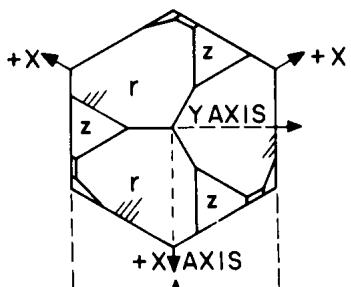
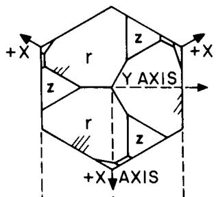
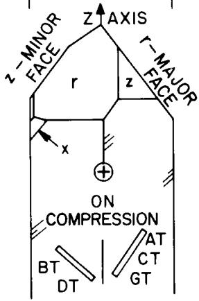
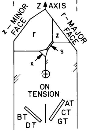
The axes according to the convention of this standard are shown in Fig 1 for right- and left-handed quartz. The conventions for handedness and sense of the axes have changed several times in the past, so the electrical and optical rules for determining these characteristics and the angular sense of common crystal cuts have been added. Briefly, the relationship of the present convention for coordinate axes to that used in IEEE Std 176-1949 is (for both right- and left-handed quartz) that the right-handed coordinate systems used in this standard are rotated about the Z-axis from the right-handed coordinate systems used in IEEE Std 176-1949. Further clarification of the sign conventions used in this standard is provided by the inclusion of Tables 6 and 7. Table 6 shows representative values of the constants in the elasto-piezo-dielectric matrices for right- and left-handed quartz. The signs shown for the and constants are consistent with the conventions of this standard. Table 7 has been included to provide an example of how the array of constants in the elasto-piezo-dielectric matrix changes under rotation of the axes, and is, for the specific case of an SC cut, made of right-handed quartz. The values for the constants used in Table 6 are taken from a publication by Bechmann [B6].
3.2.6 The Cubic System
The three equivalent axes are a, , and , often called , and . They are chosen parallel to axes of fourfold symmetry if there is no true fourfold symmetry, then parallel to twofold axes. The X, Y, and Z axes form a right-handed system parallel to the and c axes.
A positive determines the and +Y axes after any one of the axes is chosen arbitrarily as
NOTE — See note in 3.2.2.
3.3 Conventions for Axes
3.3.1 Relationship Between Crystallographic and Cartesian Axes
Axes are assigned to crystals according to Table 3, which summarizes the discussion in 3.2.1–3.2.6. Crystal classes are listed using the international system to designate the class. The method of selection of both the crystallographic axes and the rectangular axes of physics and engineering is to be read from the table. The symbols a, b, c are used for the crystallographic axes; refer to the dimensions of the unit cell along these axes; are the rectangular axes, which must always form a right-handed system, whether for a left- or a right-handed crystal. The symbols , are used for the angles between the pairs of crystallographic axes (c and b, a and and b and respectively). Both the international and the Schoenflies symbols are given, although the use of the former is preferred. In the column “International Point Groups” those classes which are piezoelectric are marked with . Under “Axis,” the numerals 2, 3, 4, 6 mean an axis of two-, three-, four-, or sixfold symmetry; (read 4 bar) means a fourfold, a sixfold axis of inversion; m or /m is a plane of symmetry perpendicular to an axis.
Table 5—Positive Sense Rules for Z, X, and Y for Trigonal and Hexagonal Crystals
| Class | +Z | +X | +Y |
| 3 | Positive $d_{33}$ | Positive $d_{11}$ | Form right-handed system |
| 32 | Arbitrary | Positive $d_{11}$ | Form right-handed system |
| 3m | Positive $d_{33}$ | Form right-handed system | Positive $d_{22}$ |
| 6 | Positive $d_{33}$ | Arbitrary | Form right-handed system |
| Form right-handed system | Positive $d_{11}$ | Positive $d_{22}$ | |
| 622 | Arbitrary | Arbitrary | Form right-handed system |
| 6mm | Positive $d_{33}$ | Arbitrary | Form right-handed system |
| 6m2 | Arbitrary | Positive $d_{11}$ | Form right-handed system |
text_image
+X r z Y AXIS r z +X AXIS
text_image
+X r z Y AXIS +X r z +X AXIS
text_image
z-MINOR FACE r z r-MAJOR FACE x + ON COMPRESSION BT DT AT CT GT
text_image
Z - MINOR FACE r z r - MAJOR FACE x + ON TENSION BT DT AT CT GT
Left-Handed Quartz
In the conoscope, z-axis rings will contract when the eyepiece is rotated clockwise. In the polariscope,the analyzer must be rotated counterclockwise to reestablish extinction.
Right-Handed Quartz
In the conoscope,z-axis rings will expand when theeyepieceis rotated clockwise. In the polariscope,the analyzer must be rotated clockwise to reestablish extinction.
Figure 1—Left- and Right-Handed Quartz Crystals, Trigonal Class 32
The procedure for determining the a, b, c axes of any crystal involves satisfying a series of conventions. The first convention is indicated under the name of each system, and gives general rules for identification of axes in terms of the relative magnitudes of the unit distances and of the angles between the crystallographic axes. With orthorhombic classes 222 and 2/m 2/m 2/m, this one rule unambiguously prescribes all crystallographic axes. With monoclinic crystals the b axis is defined in terms of the symmetry according to the third column under “Axis.” With the remaining systems, except triclinic and orthorhombic, the c axis is the first to be identified and is always the axis of high symmetry. Where the symbol † appears there is no special rule beyond that for the choice of the c axis, except that the remaining axes shall be selected in such a way as to give the smallest cell consistent with the specification of
Table 6—Elasto-Piezo-Dielectric Matrices for Right- and Left-Handed Quartz
| General form of the matrices | ||||||||
| $c^E$ in $10^9\text{ Pa}$ | ||||||||
| $e$ in $10^{-2}\text{ C/m}^2$ | ||||||||
| $\epsilon^S$ in $10^{-12}\text{ F/m}$ | ||||||||
| Right-handed quartz | ||||||||
| 86.74 | 6.99 | 11.91 | 17.91 | 0 | 0 | 17.1 | 0 | |
| 6.99 | 86.74 | 11.91 | -17.91 | 0 | 0 | -17.1 | 0 | |
| 11.91 | 11.91 | 107.2 | 0 | 0 | 0 | 0 | 0 | |
| 17.91 | -17.91 | 0 | 57.94 | 0 | 0 | 4.06 | 4.06 | |
| 0 | 0 | 0 | 0 | 57.94 | 35.82 | 0 | 0 | |
| 0 | 0 | 0 | 0 | 35.82 | 39.88 | 0 | -34.2 | |
| - | - | - | - | - | - | - | - | |
| 17.1 | -17.1 | 0 | 4.06 | 0 | 0 | 39.21 | 0 | |
| 0 | 0 | 0 | 4.06 | 0 | -34.2 | 0 | 39.21 | |
| 0 | 0 | 0 | 0 | 0 | 0 | 0 | 41.03 | |
| Left-handed quartz | ||||||||
| 86.74 | 6.99 | 11.91 | 17.91 | 0 | 0 | -17.1 | 0 | |
| 6.99 | 86.74 | 11.91 | -17.91 | 0 | 0 | 17.1 | 0 | |
| 11.91 | 11.91 | 107.2 | 0 | 0 | 0 | 0 | 0 | |
| 17.91 | -17.91 | 0 | 57.94 | 0 | 0 | -4.06 | -4.06 | |
| 0 | 0 | 0 | 0 | 57.94 | 35.82 | 0 | 0 | |
| 0 | 0 | 0 | 0 | 35.82 | 39.88 | 0 | 34.2 | |
| - | - | - | - | - | - | - | - | |
| -17.1 | 17.1 | 0 | -4.06 | 0 | 0 | 39.21 | 0 | |
| 0 | 0 | 0 | -4.06 | 0 | 34.2 | 0 | 39.21 | |
| 0 | 0 | 0 | 0 | 0 | 0 | 0 | 41.03 | |
NOTE — The matrix is the transpose of the piezoelectric matrix
Parentheses around and in columns for axis identification (tetragonal and cubic classes) indicate that the designation is arbitrary as to which of the two crystallographic axes perpendicular to c (Z) shall be X. Parentheses around (hexagonal and trigonal) indicate that any of the three a axes may be taken as X. Except for class either choice of sense may be made for the Z axis, after naming the X axis, and the choice will not affect the signs of the constants. The only restriction is that the axial system shall be right-handed. In two tetragonal classes (422 and 4/m 2/ m 2/m) and three cubic classes (432, 2/m , and 4/m 2/m) this choice is trivial in the sense that the signs, values, and matrix positions of elastic, dielectric, or piezoelectric constants are in no way affected thereby. These five classes are designated by an asterisk in the column for +/- axes.
Some nonpiezoelectric crystal classes (1, 2/m, 4/m, 3, and 3 2/m) have certain elastic constants whose signs depend upon positive sense choice for the axes. No convention is established here for a unique choice of positive sense in these cases.
The column headed “+/- Axes” indicates classes for which the sense of the axis is chosen such that given piezoelectric constants are positive.
NOTE — See note in 3.2.2.
Where two axes are listed, the choice of the third axis is such that a right-handed system results. Where only one axis is listed, the others may be chosen arbitrarily such that a right-handed system is obtained.
3.3.2 Treatment of Enantiomorphous Forms
In the eleven crystal classes (point groups) having no center of inversion or plane of symmetry, two different types of the same species may exist. Each type is the mirror image of the other, neither type can be made to look exactly like the other by a simple rotation. If the right crystal has right-handed rectangular axes, the axes of the left crystal will then appear left-handed. However, it is standard crystallographic practice to use right-handed axial systems for all crystals, whether right- or left-handed. This convention is adopted in the present standard for piezoelectricity. Under this convention, the left-handed form should be regarded as the crystallographic inversion of the right-handed form, rather than its mirror image.
Table 7—Elasto-Piezo-Dielectric Matrix for Right-Handed Quartz (YXwl) 22.4°/-33.88°
| General form of matrix | |||||||||
| $c^E$ | | | $e_t$ | $c^E$ in $10^9$ N/m2 = $10^9$ Pa | ||||||
| - | - | + | - | - | e | in $10^{-2}$ C/m2 | |||
| e | | | $\epsilon^S$ | $\epsilon^S$ in $10^{-12}$ F/m | ||||||
| +86.74 | +2.09 | +16.80 | +0.35 | +13.71 | -9.20 | +6.63 | -13.09 | -8.79 | |
| +2.09 | +115.16 | -3.72 | -8.97 | -0.93 | +19.03 | -8.33 | +9.02 | +6.06 | |
| +16.80 | -3.72 | +110.05 | -3.13 | -12.78 | -9.83 | +1.70 | +4.07 | +2.73 | |
| +0.35 | -8.97 | -3.13 | +42.31 | -9.83 | -0.93 | -1.53 | +6.06 | +4.07 | |
| +13.71 | -0.93 | -12.78 | -9.83 | +58.75 | -5.73 | -8.79 | -5.87 | -3.94 | |
| -9.20 | +19.03 | -9.83 | -0.93 | -5.73 | +39.07 | -13.09 | -2.69 | -1.81 | |
| +6.63 | -8.33 | +1.70 | -1.53 | -8.79 | -13.09 | +39.21 | 0 | 0 | |
| -13.09 | +9.02 | +4.07 | +6.06 | -5.87 | -2.69 | 0 | +39.78 | -0.84 | |
| -8.79 | +6.06 | +2.73 | +4.07 | -3.94 | -1.81 | 0 | -0.84 | +40.46 | |
NOTE — For left-handed quartz, cE and S are completely unchanged; all e terms are reversed in sign.
NOTE — The inversion operation consists of moving each point to the negative of its present position with respect to a point P called the center of inversion. An inversion is equivalent to a 180-degree rotation about any axis through P followed by reflection in a mirror perpendicular to this axis of rotation at the point P.
The eleven classes (point groups) that permit either right- or left-handed forms are triclinic 1, monoclinic 2, orthorhombic 222, tetragonal 4 and 422, trigonal 3 and 32, hexagonal 6 and 622, and cubic 23 and 432. All but 432 are piezoelectric. All eleven are included among the fifteen optically active classes.
The signs of all elastic constants are the same for left- and right-handed crystals. All piezoelectric constants, however, have opposite signs for left- and right-handed crystals.
In those classes in which enantiomorphous forms exist, the following rules identify the right-handed form for transparent crystals:
- Class 1. Right rotation of light propagating along the optic axis most nearly parallel to Z.
- Class 2. Right rotation of light propagating along the optic axis most nearly parallel to Y.
- Class 222. Right rotation of light propagating along either optic axis.
- Classes 3, 32, 6, 4, 422. Right rotation of light propagating along the Z axis.
- Classes 432, 23. Right rotation of light propagating in any direction.
NOTE — This standard assumes that left-handed is synonymous with left-rotating (levorotatory) optical activity. This may not be the case with all enantiomorphous crystals, and therefore reference to “dextrorotatory” and “levorotatory” would be more rigorous than “right-handed” and “left-handed.”
Right rotation of light occurs if the polarization vector advances in the direction of a left-handed screw. This means that in a polariscope the analyzer would have to be turned clockwise to keep the field dark if the thickness of the crystal were increased. This was described in more detail in 3.2.5.1 which defines the axes of quartz.
3.4 Elasto-Piezo-Dielectric Matrices for All Crystal Classes
A simplified presentation of the elasto-piezo-dielectric matrix for all seven crystal systems and 32 classes, using both international [B4] (Hermann-Mauguin’s) and Schoenflies’ notation (the latter in parentheses), is shown in Table 8. The tetragonal system and the trigonal system are divided into two groups designated as (a) and (b). For the tetragonal system IV(b), equals zero; for the trigonal system V(b), s25 equals zero. The 20 arrays of piezoelectric constants reduce to 16 independent arrays, since the symmetry operations for have the same effect on the piezoelectric array and the arrays for classes 23 and 3m are identical. The arrangement of the classes in Table 8 is in accordance with generally accepted practice. The numbers on the right-hand side of each array indicate, from top to bottom, the number of the independent elastic, piezoelectric, and dielectric constants.
The symmetry type of polarized polycrystalline ceramic materials, such as barium titanate or lead titanate zirconate ceramics, is associated with the crystallographic class 6mm of the hexagonal crystal system in regard to all those physical properties that are described by tensors of ranks up to four and which include dielectric, piezoelectric, and elastic phenomena.
The equations of state used to describe piezoelectric phenomena can be written in forms analogous to those used to describe piezoelectric phenomena [B7]. Piezomagnetism is not considered in this standard except to note here that the piezomagnetic matrices for specific magnetic crystal classes cannot, as a general rule, be determined from the piezoelectric matrices presented in this standard. See IEEE Std 319-1971 [8]. However, for the important cases of poled piezomagnetic and piezoelectric ceramic materials, the matrices of the effective elastic, piezomagnetic, and permeability coefficients for piezomagnetic ceramics are similar in form to the matrices of the effective elastic, piezoelectric, and dielectric coefficients for piezoelectric ceramics.
Table 9 lists crystal classes according to occurrence of piezoelectricity, pyroelectricity, optical activity, and enantiomorphism.
3.5 Use of Static Piezoelectric Measurements to Establish Crystal Axis Sense
The rules for identification of positive sense in the orthogonal X, Y, Z axes are summarized in 3.2 and 3.3. For the first axis to be identified, a positive sign is required for the first one of the following constants which does not vanish: second axis is then identified as to the sense by applying the rule to the next d constant in the group, if any, which does not vanish. Finally the last axis is chosen such that a right-handed system results. With crystals that are enantiomorphic, the rule is applied as stated to a right-handed crystal; for left-handed crystals the rule reads “negative” rather than “positive” with reference to the piezoelectric constants.
A positive value of means unambiguously that tension (accomplished by release of compression) parallel to the Z axis will cause a potential difference to be generated with its positive terminal on the +Z face, that is, the face toward which points from inside the crystal. The situation with and is identical with reference to +X and +Y, respectively. With the rule is that +Z becomes positive when a tensile stress is applied along a line 45 degrees between +X and +Y. With extension parallel to X causes +Z to become positive.
NOTE — See note in 3.2.2.
Only with triclinic class 1 and monoclinic class m crystals is it necessary to specify effectively a short-circuit measurement. With all other classes an open-circuit measurement may be used as well. For the short-circuit measurement a large linear capacitor, that is, with capacitance at least 100 times that of the test specimen, should be connected across a high-impedance voltmeter (preferably an electronic electrometer) in parallel with the test specimen. The specimen should have metal electrodes deposited on the faces upon which a potential difference is developed by the stress.
The specimen should be of such a shape that a one-dimensional compressive stress can be applied. For static conditions and the parallel d constants this means that the largest lateral dimension on the electroded face should not be more than about five times as great as the thickness. If the specimen is a square plate with edge about twice the thickness, then the mechanical condition will be one virtually free of lateral constraint, and with a large parallel capacitor all components of electric field perpendicular to the plate will be virtually zero. For a bar elongated in a direction 45 degrees between +X and +Y and with thickness parallel to Z is chosen. Under these conditions mechanical and electrical boundary conditions are satisfied. The +Z face becomes positive on release of the compressive stress applied parallel to the length of the bar. The choice of +X and +Y forms a right-handed system. For a bar elongated in the X direction and with thickness parallel to Z is chosen. The +Z face becomes positive on release of compressive stress applied parallel to the length of the bar. The potential generated across the capacitor is positive on the terminal connected on the positive end of the axis upon release of compression, negative upon compression.
Table 8—Elasto-Piezo-Dielectric Matrices for the 32 Crystal Classes*
*The numbers on the right-hand side of each scheme indicate, from top to bottom, the numbers of the independent elastic, piezoelectric, and dielectric constants.
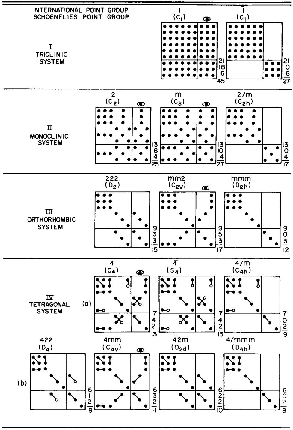
table
| System | Group | Value |
|---|---|---|
| INTERNATIONAL POINT GROUP SCHOENFLIES POINT GROUP | I (C₁) | 21/18/6/45 |
| INTERNATIONAL POINT GROUP SCHOENFLIES POINT GROUP | T (C₁) | 21/0/6/27 |
| II MONOCLINIC SYSTEM | 2 (C₂) | 13/8/4/25 |
| II MONOCLINIC SYSTEM | m (Cₛ) | 13/10/4/27 |
| II MONOCLINIC SYSTEM | 2/m (C₂h) | 13/0/4/17 |
| III ORTHORHOMBIC SYSTEM | 222 (D₂) | 9/3/3/15 |
| III ORTHORHOMBIC SYSTEM | mm2 (C₂v) | 9/5/3/17 |
| III ORTHORHOMBIC SYSTEM | mmm (D₂h) | 9/0/3/12 |
| IV TETRAGONAL SYSTEM (a) | 4 (C₄) | 7/4/2/13 |
| IV TETRAGONAL SYSTEM (a) | 4̅ (S₄) | 7/4/2/13 |
| IV TETRAGONAL SYSTEM (a) | 4/m (C₄h) | 7/0/2/9 |
| 422 (D₄) | 4mm (C₄v) | 6/2/9 |
| 422 (D₄) | 42m (D₂d) | 6/2/11 |
| (b) | 6 (C₄v) | 6/3/2/11 |
| (b) | 6 (D₂d) | 6/2/10 |
| (b) | 6 (D₄h) | 6/0/8 |
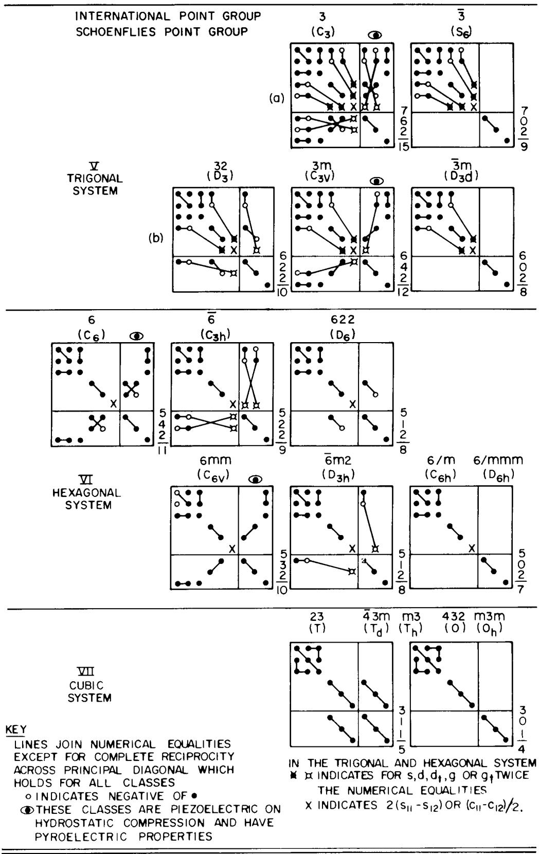
KEY
LINES JOIN NUMERICAL EQUALITIES EXCEPTFOR COMPLETERECIPROCITY ACROSS PRINCIPALDIAGONAL WHICH HOLDS FOR ALL CLASSES OINDICATES NEGATIVE OF·
THESECLASSES ARE PIEZOELECTRIC ONHYDROSTATIC COMPRESSION AND HAVEPYROELECTRIC PROPERTIES
IN THE TRIGONAL AND HEXAGONAL SYSTEM XINDICATES FOR THE NUMERICAL EOUALITIES X INDICATES
Table 9—Occurrence of Piezoelectricity, Pyroelectricity, Optical Activity, and Enantiomorphism
| Crystal System | Piezoelectric Classes | Pyroelectric Classes | Classes with Optical Activity* | Classes with Enantiomorphism |
| Triclinic | 1 | 1 | 1 | 1 |
| Monoclinic | 2, m | 2, m | 2, m | 2 |
| Orthorhombic | 222, mm2 | mm2 | 222, mm2 | 222 |
| Tetragonal | 4, 4, 4224mm, 42m | 4, 4mm | 4, 4224, 42m | 4, 422 |
| Trigonal | 3, 32, 3m | 3, 3m | 3, 32 | 3, 32 |
| Hexagonal | 6, 6, 6226mm, 6m 2 | 6, 6mm | 6, 622 | 6, 622 |
| Cubic | 23, 43m | None | 23, 432 | 23, 432 |
*Point groups that can have nonzero components of the gyration tensor [B8] are defined as optically active. However, for uniaxial materials only those point groups that allow enantiomorphism can exhibit optical rotation of polarized light propagating along the optic axis. This affects only classes 4 and 42m.
NOTE — See note in 3.2.2.
Care must be taken not to be confused by pyroelectric charges generated by temperature drift with polar crystals. If the compressive stress is applied, stabilized to a nearly neutral condition, and then released rather suddenly, piezoelectrically generated charges usually far exceed pyroelectrically generated charges. Care must also be taken to apply a stress as nearly parallel to the desired axis as possible. Therefore faces perpendicular to this axis should preferably be flat and parallel.
3.6 System of Notation for Designating the Orientation of Crystalline Bars and Plates
3.6.1 General
A crystal plate cut from a single-crystal starting material can have an arbitrary orientation relative to the three orthogonal crystal axes X, Y, and Z. The rotational symbol provides one way in which the plate of arbitrary orientation can be specified. The rotational symbol uses as a starting reference one of three hypothetical plates with thickness along X, Y, or Z, and then carries this plate through successive rotations about coordinate axes, fixed in the reference plate, to reach the final orientation.
Since rectangular plates are frequently used, the symbols l, w, and t denote the length, width, and thickness of the plate; we use the notation l, w, t to denote the orthogonal coordinate axes fixed in the reference plate. The rotational symbol is defined by the convention that the first letter (X, Y, or Z) indicates the initial principal direction of the thickness of the hypothetical plate and the second letter (X, Y, or Z) indicates the initial principal direction of the length of the hypothetical plate. The remaining letters of the rotational symbol indicate the successive edges of the hypothetical plate used as successive rotation axes. Thus the third letter (l, w, or t) denotes which of the three orthogonal coordinate axes in the hypothetical plate is the axis of the first rotation, the fourth letter (l, w, or t) the axis of the second rotation, the the fifth letter (l, w, or t) the axis of third rotation. Consequently, if one rotation suffices to describe the final orientation of the plate, there are only three letters in the symbol, and if two rotations suffice, there are four letters in the symbol. Clearly, no more than five letters are ever needed to specify the most general orientation of a plate relative to the crystal axes by means of the rotational symbol. The symbol is followed by a list of rotation angles F, Q, Y, each angle corresponding to the successive rotation axes in order. The specification of negative rotation angles consists of the magnitude of the angle preceded by a negative sign. An angle is positive if the rotation is counterclockwise looking down the positive end of the axis toward the origin. Thus an example of the rotational symbol for the most general type of rotation might be
which means that initially the thickness and length of the hypothetical plate are along the Y and X axes, respectively, the first rotation of amount F is about the l axis, the second rotation of amount Q about the w axis, and the third rotation of amount Y about the t axis. As a specific example, consider the following:
This is a specification for a plate whose thickness was initially chosen along the Y axis and the length along the Z axis. The plate was then rotated successfully about its thickness, about its width, and about its length. A statement of the magnitude of w completes the specification for a prescribed plate or bar. If the final plate or bar is other than rectangular (that is, round or irregularly shaped), then the l and w axes must be given as specific defined orthogonal axes in the plane of the plate, at least one of which must be noted on the actual plate. If the plate is square, one axis in the plane of the plate is specifically identified as l and the other as w.
3.6.2 Nonrotated Plates
Figure 2 shows two examples of nonrotated cuts. Note that only two letters are needed in the rotational symbol. Practically all the commonly used flexural and extensional mode (except the NT-cut) quartz resonators may be obtained by a single rotation of the (XY) plate. Practically all the commonly used thickness and face-shear mode quartz resonators may be obtained by a single rotation of the (YZ) plate.
3.6.3 Singly Rotated Plates
Practically all of the commonly-used flexural and extensional mode (except the NT-cut) quartz resonators may be obtained by a single rotation of the (XY) plate. Practically all the commonly used thickness-shear and face-shear mode (except the SC-cut) quartz resonators may be obtained by a single rotation of the (YZ) plate. Figure 3 shows an example of a singly rotated plate, in this case the commonly known AT cut. (Actually, the AT cut represents a family of cuts where the precise value of the angle Q varies by as much as ±1°, depending upon the details of the starting material and the specific application.) In Fig 3, the plate has its length along the digonal (or X) axis and has the rotational symbol . A BT-cut quartz plate with its length along the digonal axis has the rotational symbol (YXl) 49°. An example of this cut is shown in Fig 4.
3.6.4 Doubly Rotated Plates
Figure 5 shows an example of a doubly rotated plate, in this case the GT cut. The rotational symbol has four letters followed by two angles and is given by . Another example of a doubly rotated cut is given in Fig 6, which shows an SC cut. In this case, the rotational symbol that is used to specify the cut is (YXwl) 22.4°/-33.88°. As in the case of the AT cut, the cut as shown here actually represents a family of cuts where the ranges in the angles F and Q are ±2° in F and in again depending upon the starting material and the specific application.
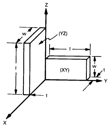
text_image
Z (YZ) l (XY) w t Y t X t w
Figure 2—Examples of Nonrotated Plates
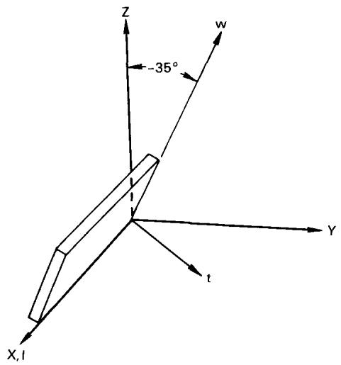
text_image
-35° Z w Y t X,I
Figure 3—Illustration of an AT-Cut Quartz Plate Having the Notation (YXl)
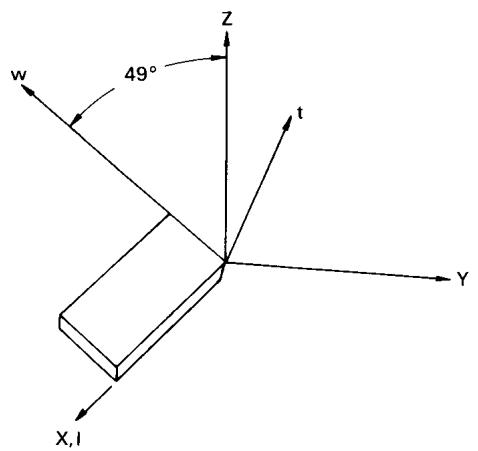
text_image
w 49° Z t Y X,1
Figure 4—Illustration of a BT-Cut Quartz Plate Having the Notation (YXl)
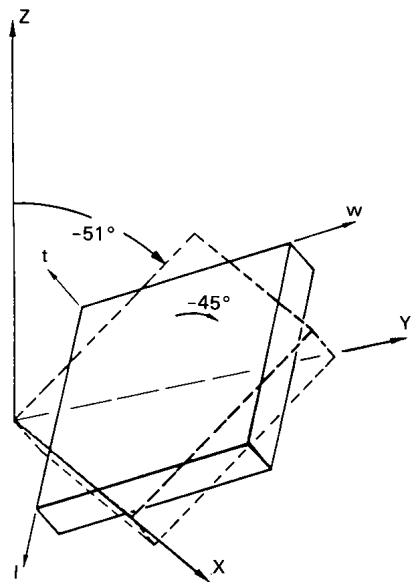
text_image
Z -51° t -45° W Y X
Figure 5—Illustration of a Doubly Rotated Quartz Plate, the GT Cut, Having the Notation (YXlt)-51°/-45°
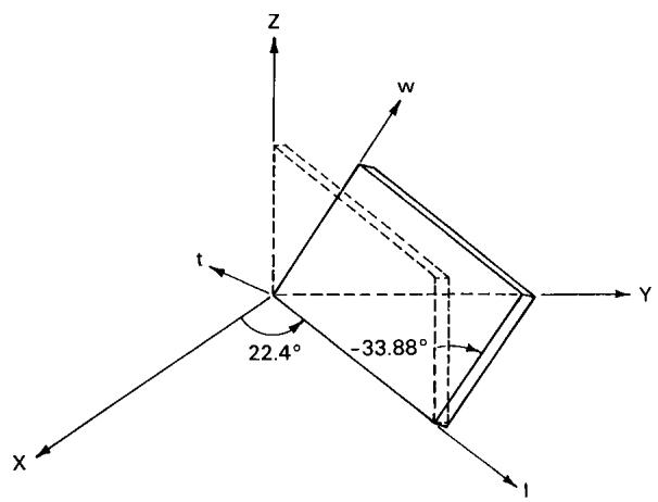
text_image
Z w Y t 22.4° -33.88° X l
Figure 6—Illustration of a Doubly-Rotated Quartz Plate, the SC Cut, Having the Notation (YXwl) 22.4°/-33.88°
3.6.5 Triply Rotated Cuts
While no triply rotated bars or plates have found substantial applications, the rotational symbol provides for their use, and the specification may be derived by an extension of the methods illustrated.
4. Wave and Vibration Theory
4.1 General
Those interested in laboratory measurements only can omit this section. However, this section contains many cautionary statements and is required for the description of certain thickness vibrators and extensional and cylindrical resonators.
This section considers steady-state propagating and standing-wave solutions of the system of equations presented in Section 2. These solutions are readily obtainable, provide much valuable information, and form the basis for many of the equations used in connection with the measurements in Section 6.. In particular, plane-wave solutions for the arbitrarily anisotropic, infinite piezoelectric medium are presented, and, as examples of the general theory, are specialized to the cases of propagation along a particular principal direction for the somewhat similar crystal classes 32 and 3m. The, differences in the propagation characteristics are discussed for the particular principal direction considered in the two crystals. The solutions for the frequencies of resonance and antiresonance for the thickness vibrations of an arbitrarily anisotropic piezoelectric plate driven by electrodes on either the major (thicknessexcitation) or minor (lateral-excitation) surfaces of the plate are presented. In the case of thickness excitation of thickness vibrations the general solution is applied to the special cases of Y-cut plates in the crystal classes 32 and 3m, and it is shown that although a single piezoelectric coupling factor can be defined for the Y cut of crystal class 32, one cannot be defined for the Y cut of crystal class 3m. The frequency equation for the thickness resonances under thickness excitation in the general anisotropic case is shown to simplify considerably when the piezoelectric coupling is small.
The approximate equations for the low-frequency extensional motion of anisotropic piezoelectric rods of rectangular cross section are presented. The three different possible placements of driving electrodes on entire rectangular surfaces are discussed. The solutions for the frequencies of resonance and antiresonance of the extensional modes of the rods are presented for each of the three cases. The pertinent approximate equations for the low-frequency radial motion of thin circular plates in crystal class or the subclasses , with the fully electroded circular surfaces normal to the three- or sixfold axes are presented. The solution for the frequencies of resonance and antiresonance of the radial modes of the thin circular plate are presented.
4.2 Piezoelectric Plane Waves
For plane-wave propagation in the infinite medium, Eq 20 and Eq 21 may be combined to give ([B2], Eq 9.51)
where
denotes the piezoelectrically stiffened elastic constants for plane-wave propagation in the direction where denotes the magnitude of length in the propagation direction and the components of the unit wave normal relative to the crystal axes, and the convention that a repeated Greek index is not to be summed has been adopted. When the second term in Eq 47 vanishes, the elastic constant is said to be unstiffened.
Steady-state plane-wave solutions of Eq 46 may be written
where represents the amplitude of each displacement component. From Eqs 46 and 48 the three wave velocities for the direction may be found from the three assumed-positive eigen-values (n) of
by means of the relation
The displacement directions of the three waves are orthogonal because of the symmetry of . However, in general, the three waves have displacement vectors that are neither parallel nor perpendicular to the propagation direction. Nevertheless, for certain special directions in crystals possessing some symmetry, there may be a longitudinal and two transverse waves or one transverse wave and two mixed waves. These purely longitudinal or purely transverse waves, which propagate along certain symmetry directions, are frequently of significant practical value. As examples of the foregoing general treatment, a specific propagation direction in both quartz (class 32) and lithium niobate (class 3m), which have some similar and some different features, are treated in this section.
The arrays of constants referred to the crystal axes [XYZ], which in this section are denoted by for a crystal in class 32, may be obtained from Table 8. For propagation in the direction, Eq 49 takes the form
where, from Eq 47,
is the piezoelectrically stiffened elastic constant for propagation in the direction for crystals in class 32. Eq 51 shows that in this case there are one stiffened piezoelectric shear wave and two purely elastic waves, each of which has components of mechanical displacement normal and transverse to the direction of propagation.
The arrays of constants referred to the crystal axes for materials in crystal class 3m may be obtained from Table 8. For propagation in the direction, Eq 49 takes the form
where the piezoelectrically stiffened elastic constants may be determined from Eq 47 in the same way as Eq 52. Eq 53 shows that in this case there are one unstiffened purely elastic shear wave and two stiffened piezoelectric waves which have coupled longitudinal and transverse motions.
In the same manner, Eq 49 can be used to find the plane-wave propagation properties for any orientation in any piezoelectric crystal.
4.3 Thickness Excitation of Thickness Vibrations
NOTE — This section deals only with the lossless resonator. In this case the phase of the admittance or the impedance is always ± /2. The frequency commonly identified as the resonance frequency is the lower of the pair of critical frequencies identified in this standard as and . The lower critical frequency is defined as the frequency of maximum admittance for the lossless resonator). The upper critical frequency is defined as the frequency of maximum impedance for the lossless resonator) and in this section, as well as in common practice, this will be called the antiresonance frequency. These definitions are used to avoid confusion with the definitions of IEEE Std 177-1978 [5]. In Section , which deals with measurements on real materials, it is explained tha corresponds and, under certain conditions, corresponds
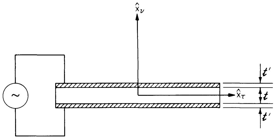
text_image
Diagram illustrating a physical or mathematical model with labeled axes, variables, and time intervals
Figure 7—Thickness Excitation of a Plate
A schematic diagram of the piezoelectric plate is shown in Fig 7. The anisotropic plate of thickness t is driven by the application of an ac voltage across electrodes of thickness on the major surfaces, and the other dimensions are sufficiently larger than t that the boundary conditions on the minor surfaces can be ignored [B9]. The resonance frequencies are given by the roots of the determinantal equation ([B2], Eq 9.69, and Chapter 16, Section 3.)
where the are the components of the unit eigenvectors associated with each eigenvalue (n) of Eq 49 for the direction and
and is the density of the plate material, the electrode density, and the circular frequency.
The quantity R is a consequence of the inertia of the electrode plating. Eq 54 is a transcendental determinant, each term of which is very complicated. Eq 54 can be put in a simpler, more compact form, which is useful for many purposes, and results directly from the expression for the electrical admittance of the oscillating crystal. For the admittance is given by
where A is the area of one electroded surface of the plate, and
From Eq 56 the resonance frequencies of the oscillating crystal plate are given by the roots of the transcendental equation ([B2], Eq 9.77)
It should be noted that Eqs 54, 56, and 58 are valid only when the thickness of the electrode is much less than a wavelength, which condition can be written in the form
Either Eq 54 or Eq 58 shows that, in general, all three plane-wave solutions for the direction , discussed in 4.2, are coupled by the boundary conditions at the conducting surfaces of the plate at resonance. Nevertheless, for certain orientations of crystal plates with certain symmetries, major simplifications in Eqs 54 and 58 result.
When the electrode inertia is negligible (R@0), the admittance, Eq 56, for an arbitrarily anisotropic crystal resonator (with its major surfaces electroded) approaches zero for
which thus defines the antiresonance frequency
At that condition there is no coupling between the three different plane-wave solutions for the direction . Eq 60 also serves as a frequently useful approximation for the resonance frequency at any overtone, for materials with small and even for materials with large k at higher (³7) overtones, where is very large. Eventually, however, a point is reached beyond which the electrode inertia R is no longer negligible, and the relations 59 and 60 are no longer valid. Moreover, if the overtones are sufficiently high that the wavelength is of the order of , even Eqs 54, 56, and 58 cease to be valid.
As examples of the foregoing general treatment, a specific orientation of both a plate of quartz (class 32) and a plate of lithium niobate (class 3m) are treated in this section. In the case of Y-cut quartz, the symmetry results in a major simplification of Eqs 54 and 58 while in the case of Y-cut lithium niobate the symmetry does not result in a major simplification of Eqs 54 and 58. In both cases, the influence of electrode inertia is ignored—that is, is assumed to vanish.
The orientation of the crystal axes of a crystal in class 32 with respect to the coordinate axes is the same as in 4.2. For Y—cut quartz, the electroded surfaces of the plate are normal to the direction, = 2, and as a consequence of the form of Eq 51 is not diagonal. Nevertheless, since the off-diagonal terms affect only purely elastic terms, Eq 58 yields the transcendental equation
In Eq 61, is the thickness-shear piezoelectric coupling factor for a Y cut of the material and is given by
In addition to Eq 61, Eq 54 yields the two transcendental equations
which govern two sets of purely elastic modes that cannot be driven electrically by a perfect thickness excitation, and are not contained in the admittance relation Eq 56 because Eq 56 automatically excludes modes undriven electrically. The transcendental equation (Eq 61) governs the set of piezoelectric thickness-shear modes which are driven electrically by a perfect thickness excitation. The form of 61 shows that the resonance frequencies are not integral multiples of the fundamental [B10].
Lithium niobate, lithium tantalate, and tourmaline are among the crystals in class 3m. The orientation of the principal axes of a crystal in class 3m with respect to the coordinate axes is the same as in 4.2. For a Y cut the electroded surfaces of the plate are normal to the direction, = 2, and as a consequence of the form of Eq 53, is not diagonal. In this case the off-diagonal terms affect piezoelectrically stiffened terms and, as a consequence, Eq 58 yields the transcendental equation
where
In addition to Eq 64, Eq 54 yields the transcendental equation
which governs a set of purely elastic thickness-shear modes that cannot be driven electrically by a pure thickness excitation, and is not contained in the admittance relation Eq 56. The transcendental equation (Eq 64) governs the set of piezoelectric coupled shear and extensional modes which are driven electrically by a perfect thickness excitation. Eq 64 contains two dimensionless material coefficients and , thereby showing that the two piezoelectrically stiffened standing waves are coupled at the conducting surfaces for this principal orientation of the crystal plate. However, although the lower modes must be determined analytically from the roots of Eq 64, the high overtones (seventh and higher) are essentially elastic and may be determined from the roots of Eq 59. Moreover, for low coupling materials, Eq 64 can usually be approximated by
unless the material constants are such that is not very different from , or they bear some unusual relationship to each other. In addition, for high coupling materials, the material constants may be such that there may be a few orientations for which Eq 64 may be approximated by Eq 67. However, such orientations are best found analytically after the fundamental material constants are determined from appropriate measurements [B11]. In any event the are not simple combinations of the material constants as is in Eq 62, but are given by the complicated combination of the material constants shown in Eq 65.
When the transcendental equation (Eq 54) factors into three separate parts, such as those shown in Eqs 61 and 63 (where electrode inertia is ignored), and electrode inertia is included, the transcendental equation governing the set of piezoelectric thickness modes may be written in the form ([B2], Chapter 16, Section 3.)
in place of the form shown in Eq 61. An equation similar to Eq 68 holds in all other analogous cases discussed in this section.
When the piezoelectric coupling factor is small, that is, , as well as the electrode inertia, that is, , and Eq 68 is valid, we may write ([B2], Chapter 16, Section 3.)
for particular values of i and From Eq 69 for the resonance frequency and the condition for antiresonance, Eq 60, the difference in frequency Df between the lowest antiresonance and resonance is given by
for small and R.
In the same manner, Eq 58 can be used to find the thickness vibrations of any orientation of any thickness excited crystal plate.
4.4 Lateral Excitation of Thickness Vibrations
A schematic diagram of the piezoelectric plate is shown in Fig 8. The anisotropic plate of thickness t is driven by the application of an ac voltage across electrodes on one pair of minor surfaces, which are taken normal to The length and width to thickness ratios are sufficiently large that the boundary conditions on the minor surfaces can be ignored [B9], and the solution obtained for regions distant from the minor surfaces. For this case the electrical admittance per unit width is given by
where
and
and the are the components of the unit eigenvectors associated with each eigenvalue of
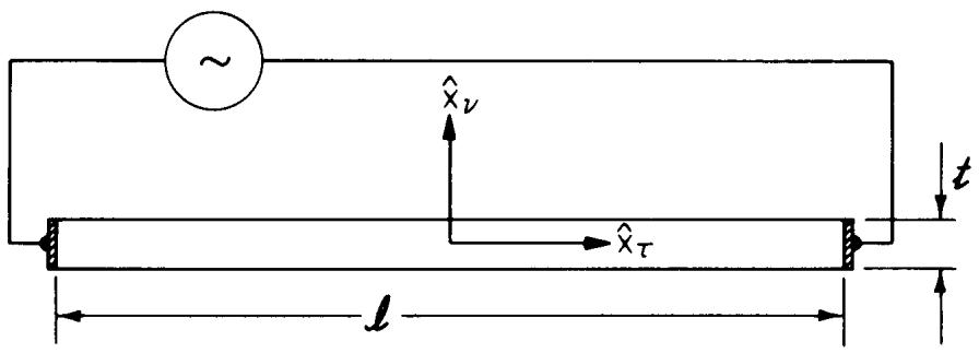
text_image
~ x̂_v t x̂_τ l
Figure 8—Lateral Excitation of a Plate
Eq 49 for the direction and are defined in Eq 55, and the driving field between the electrodes has been assumed uniform. From the resonance frequencies are given by the roots of the transcendental equation
and the resonance frequencies may be determined from the relation
Thus when the major surfaces are nonconducting, the piezoelectric standing-wave solutions of the differential equations are not coupled at thickness resonance.
From Eq 71 the antiresonance frequencies for lateral excitation of thickness vibrations are given by the roots of the transcendental equation
Eq 76 shows that in general the three piezoelectric standing-wave solutions are coupled at thickness antiresonance for lateral excitation. At high overtones Eq 76 may be approximated by Eq 74. When symmetry is present, can frequently be simplified considerably. The simplifications are analogous to those discussed in 4.3. Lateral excitation is of practical value as a method of electrically exciting unstiffened purely elastic thickness modes, from which certain elastic constants may be determined from resonance measurements when appropriate symmetry exists [B11]. Consequently, the antiresonance solution is of no particular importance, and simplifications in Eq 76 for particular symmetries will not be discussed in this standard. Moreover, since the symmetry required for the lateral electrical excitation of purely elastic thickness modes is directly related to the measurement program for the determination of all the material constants for a particular crystal, discussion of some of these special modes is given in the section on measurements, Section 6., where it more properly belongs.
4.5 Low-Frequency Extensional Vibrations of Rods
In the approximate equations for the low-frequency extensional motions of anisotropic piezoelectric rods of rectangular cross section, three distinct cases have to be distinguished. These three cases have to do with the placement of the driving electrodes relative to the cross-sectional geometry. In Fig 9 a rectangular rod of length l, thickness t, and width w is shown, where » w and . In the figure the arbitrary coordinate axis 1 , relative to the crystal axes, is directed along the rod axis, in the thickness direction, and in the width direction. In the low-frequency extensional motion of thin rods it is appropriate to take the vanishing boundary stresses on the surfaces bounding the two small dimensions to vanish everywhere. Consequently, in all three cases all vanish except . However, the electrical conditions are different in each case.
If the surfaces of cross-sectional area lw are fully electroded, the appropriate electrical conditions are everywhere, and the pertinent constitutive equations are
where
and V is the driving voltage; the carets have been placed on the constants to indicate that the constants are referred to the coordinates , and the compressed matrix notation has been employed. The pertinent differential equation and boundary conditions are
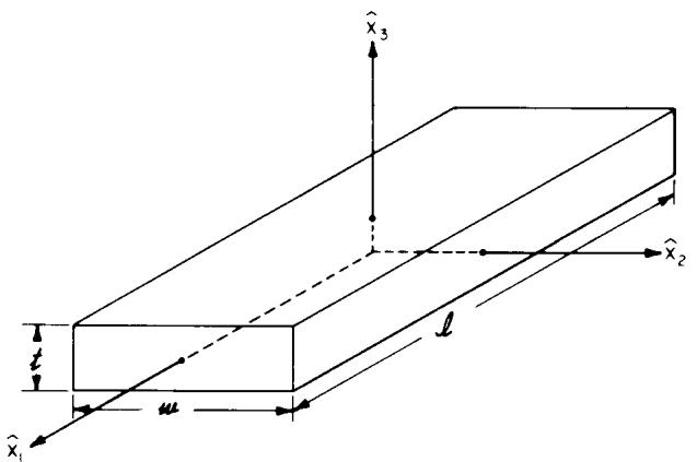
text_image
t w l x̂₁ x̂₂ x̂₃
Figure 9—A Rectangular Bar Positioned in a Cartesian Coordinate System
The electrical admittance for is given by
where
and is one of the rod extensional piezoelectric coupling factors, and is given by
From Eq 82 the resonance frequencies are given by the roots of the transcendental equation
and the resonance frequencies may be determined from the relation
From Eq 82 the antiresonance frequencies are given by the roots of the transcendental equation
If the surfaces of cross-sectional area lt are fully electroded, the appropriate electrical conditions are and 0 everywhere, and the pertinent constitutive equations are
where
and
In this case the pertinent differential equation is obtained by replacing by in Eq 80, and the pertinent boundary conditions are given by Eq 81, and it has been assumed that is much greater than the dielectric constant of the surrounding medium. Consequently Eqs 82–87 remain valid provided w and t are interchanged, is replaced by by by , by , and by .
If the surfaces of cross-sectional area wt are fully covered by an electrode, the appropriate electrical conditions are everywhere, and the pertinent constitutive equations are
The pertinent differential equations and boundary conditions are
where is the amplitude of the driving voltage. In this latter case it has been assumed that the dielectric constants of the material are considerably greater than the dielectric constant of the surrounding medium, and it is not essential that the w/t relation be adhered to, or even that the rod have a rectangular cross section. It should be noted that in all three cases the and requirements become more stringent as the piezoelectric coupling increases.
The electrical admittance is given by
where
and
From Eq 96 the resonance frequencies are given by the roots of the transcendental equation
From 96 the antiresonance frequencies are given by the roots of the transcendental equation
and may be determined from 86 provided is replaced by .
When the piezoelectric coupling factor for rods is small, the expression
holds, where is the difference between the lowest frequency of antiresonance and resonance.
4.6 Radial Modes in Thin Plates
A schematic diagram of a thin circular plate of a material in crystal class or the subclasses which include the polarized ceramic, with the circular surfaces normal to the three- or sixfold axis is shown in Fig 10. The major surfaces of the plate are fully covered by electrodes. The coordinate axis is directed normal to the circular surfaces in which r and are measured. The plate is driven into radial vibration by the application of an ac voltage across the surface electrodes. The differential equation for radial motion of the disk is [B12]
where is the radial component of displacement and
The pertinent constitutive equations are
where [B12], [B13]
and
where V is the driving voltage. The nontrivial boundary condition for the planar radial modes is
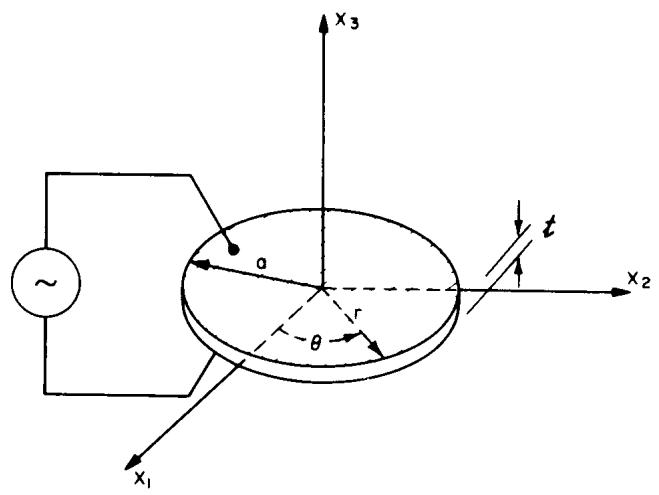
text_image
x₃ a r θ t x₂ x₁
Figure 10—Radial Mode Excitation of a Circular Disk
The steady-state forced vibrational solution of Eq 102, and satisfying Eq 108, may be written in the form
where is the driving frequency, is the Bessel function of the first kind and first order, and
The electrical admittance is given by
where is the modified quotient of cylinder functions [B14] of the first order, defined by
and is the Bessel function of the first kind and zero order,
and may be interpreted as a planar Poisson’s ratio. The coefficient is a planar radial piezoelectric coupling coefficient for the thin circular polarized ceramic disk and is given by
It is related to the usual planar coupling factor by the relation
and, where is related to , by the well-known relation
Combining Eqs 106, 111, and 115,
From Eq 111 the resonance frequencies are given by the roots of the transcendental equation
From Eq 111 the antiresonance frequencies (Y= 0) are given by the roots of the transcendental equation
When the planar piezoelectric coupling factor is small, the expression
holds, where Df is the difference between the lowest frequency of antiresonance and resonance, and , the lowest root of
5. Simple Homogeneous Static Solutions
5.1 General
The characterization of a piezoelectric body is simplified considerably under static conditions and at low frequencies far removed from its lowest elastic resonance. In the general case there could nevertheless be fairly complicated distributions of strain and electric field. The usual case and the one considered here is, however, homogeneous—that is, the strains and electric field are independent of position. Quasistatic flexure involves nonuniform strain and is therefore not considered here.
Static and quasistatic measurements or applications are practical only with piezoelectric materials having high permittivity and low conductivity. For the direct effect low permittivity requires an extremely high impedance electric load, and conductivity causes internal leakage. For the converse effect conductivity constitutes a power drain, and with low-permittivity piezoelectrics mechanical strains are low. Static and quasistatic measurements and applications are thus generally considered only with ferroelectrics, primarily the piezoelectric (poled ferroelectric) ceramics. With these, the product of volume resistivity and permittivity is generally over seconds, and relative permittivities range from 200 to 3500 at room temperature.
5.2 Applicable Equations
Although Eqs 37 and 38 are valid in a strict sense only when the and are constants, the equations are For the applications of interest in this section, from Eq 37, set
for an increment of electric displacement at constant . The use of this procedure makes it possible to obtain values of from experimental procedures discussed in this section. When the are constant, the experimental curves are straight lines as shown in Fig 11(a) and (b), and the slope of the straight line in either figure determines the value of that particular Typical experimental curves for variable are shown in Fig 11(c) and (d), and the values of a particular ) may be determined from the slopes of these curves. When the material coefficients are constant, the procedure is completely justified. However, when the material coefficients vary, it should be noted that even though the procedure is not obtained from a proper nonlinear description, it turns out to be useful for correlating experimental data under the aforementioned circumstances.
NOTE — For proper nonlinear descriptions in existence in the open literature see [B15].
In view of these considerations, the piezoelectric constant may in the static case be determined by measurement of the strain developed as a result of an applied field at constant stress. Alternatively, the charge density developed by an applied stress may be measured at constant electric field. All piezoelectric d constants in which and may be measured directly using bars or plates with edges oriented along XYZ. Details of measurement schemes for face shear and thickness shear d constants are given in 6.4.5 and 6.4.7, respectively. The simple characterization of piezoelectric elements involves the d constants for low-frequency and static applications and the e constants for high-frequency applications. Since matrix inversion involves considerable multiplication of measurement errors, it is recommended that the set of e constants not be derived from the set of d constants, but rather be measured directly, using procedures outlined in 4.3 and 6.4.7.
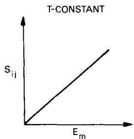
line chart
| Em | Sij |
|---|---|
| 0 | 0 |
(a)
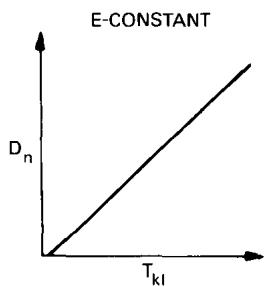
line chart
| T_kl | D_n |
|---|---|
| 0 | 0 |
(b)
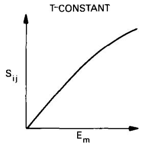
line chart
| Em | Sij |
|---|---|
| 0 | 0 |
| >0 | >0 |
(c)
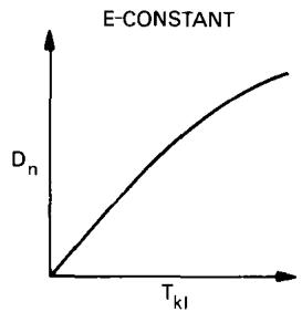
line chart
| T_kl | D_n |
|---|---|
| 0 | 0 |
| >T_k1 | Increasing trend from D_n to near 1 |
Figure 11—Schematic Illustration of Linear and Nonlinear Piezoelectric Behavior (a), (b) Constant (c), (d) Variable
The boundary conditions described for low-frequency or static measurements are summarized below:
- For measurement of constant stress, only one component of electric field changing.
- For measurement of constant electric field, only one component of stress changing.
These conditions may be achieved readily with proper attention. For (1) it is necessary only that there be no change in stress and that be the only time-dependent component of electric field. This is readily accomplished in the static or low-frequency case by maintaining a condition of zero stress and applying the electric field parallel to a dimension small with respect to the lateral electrode dimensions. For measurements of the type , the bar should be relatively long and the thickness small.
NOTE — Where specific electroelastic coefficients are listed in this section, the matrix notation introduced in 2.4 is used.
For measurements of the type , experience shows that the lateral dimensions should be about twice the thickness; this represents a compromise between boundary condition requirements (with rotated cuts or for classes 1 and m) and mechanical displacement measurement accuracy.
For (2) the presence of only one time-dependent stress component is assured by the absence of stress other than that provided to produce the stress that is, cross expansion can occur readily. The electric field is maintained constant (at very close to zero) by a capacitor with at least times the capacitance of the specimen across its electroded terminals is sufficient for the practical case where higher sensitivity is required). For all crystal classes except 1 and m, all components of the electric field will be zero for cuts oriented along the X, Y, and Z axes. With crystal classes 1 and m, all components of the electric field will be zero only if the electroded face is perpendicular to one of the three principal axes of the dielectric ellipsoid. If the direct effect is to be used for the measurement of piezoelectric constants of crystals in classes 1 and it is necessary that the thickness be small compared to the lateral electrode dimensions. However, note that the technique can not be used for specimens in class m that are electroded on Y faces, because is zero. A reasonable compromise for measurements of the type is to have a lateral dimension twice the thickness dimension. This assures reasonable freedom from lateral mechanical and electrical constraint. For measurements of the type the bar should be long, parallel to the applied stress, and thin between electrodes.
Unless the piezoelectric element is only partially electroded, is subjected to a stress such that flexure results, or is subject to specific lateral constraint, the strain and electric field are homogeneous for the static and low-frequency cases. The situation is somewhat more complex, for instance, with a piezoelectric bender. The convex side of the bender is under tension and the concave side is under compression, and a point of zero stress exists in an intermediate layer. There is also a distribution of stress along the length of the bender. In all the discussions in Section 5., only configurations with a homogeneous distribution of strain and electric field are considered.
5.3 Applicability of Static Solutions in the Low-Frequency Range (Quasistatic)
Static solutions may be used not only for the strictly static case but also over a frequency range below which there is no appreciable spatial variation in stress or electric field. The specific range depends somewhat upon the mechanical of the specimen, but in general the error will be less than 1% and 0.1%, respectively, if the frequency is less than one tenth or 0.03 times the lowest resonant frequency of the specimen.
The low-frequency range specified extends into the kilohertz range except for large specimens. As an alternative to resonance methods quasistatic measurements of piezoelectric constants are more convenient than purely static measurements because of a more favorable impedance level and elimination of anomalous factors such as pyroelectric response in polar crystals. Accuracy is better, however, using resonance methods. These are described in 6.4.
5.4 Definition of Quasistatic Material Coupling Factors
Characterization of piezoelectric crystals and ceramics can be accomplished through the piezoelectric, dielectric, and elastic tensors, including all alternate forms described in 2.6. The coupling factors are nondimensional coefficients which are useful for the description of a particular piezoelectric material under a particular stress and electric field configuration for conversion of stored energy to mechanical or electric work. The coupling factors consist of particular combinations of piezoelectric, dielectric, and elastic coefficients. Since they are dimensionless, it is clear that the coupling factors serve to provide a useful comparison between different piezoelectric materials independent of the specific values of permittivity or compliance, both of which may vary widely.
Figure 12 serves to illustrate graphically the meaning of the coupling factor for the value 0.70 typical for a piezoelectric ceramic. The element is plated on faces perpendicular to , the polar axis, and it is short-circuited as a compressive stress is applied [Fig 12 (a)]. The element is free to cross expand so that is the only nonzero stress component. From the figure it can be seen that the total stored energy per unit volume at maximum compression is + . Prior to removal of the compressive stress, the element is open-circuited. It is then connected to an ideal electric load to complete the cycle. As work is done on the electric load, the strain returns to its initial state. For the idealized cycle illustrated, the work done on the electric load and the part of the energy unavailable to the electric load are related to the coupling factor as follows:
Figure 12(b) illustrates conversion of energy obtained from an electrical source to mechanical work. The element is mechanically free when the electric source is connected. Then the element is blocked mechanically parallel to before the electric source is disconnected. Then with the mechanical block is removed and in its place a finite mechanical load is provided. For this idealized cycle the work delivered to the mechanical load and the part of the energy unavailable to the mechanical load are related to the coupling factor as follows:
Under static or quasistatic conditions, the spatial distribution of the strain and electric fields is uniform, and it is possible to define coupling constants of a material for a particular stress and electric field configuration. These are termed material coupling factors. For certain crystal classes and certain configurations, it is not possible to have a simple resonant mode. It should be noted that not every quasistatic coupling factor corresponds to a coupling factor for a piezoelectric mode discussed in 6.4.
Table 10 lists important static and quasistatic coupling factors with appropriate mechanical conditions. Other coupling factors can be defined for other sets of boundary conditions, but those listed are the important ones.
5.5 Nonlinear Low-Frequency Characteristics of Ferroelectric Materials (Domain Effects)
Deviations from linear behavior which occur with ferroelectrics are due to mechanical and electrical influences on domain configurations. This will not be discussed in detail here. It should, however, be noted that such nonlinearities are most pronounced under static and quasistatic conditions. Static and quasistatic measurements of piezoelectric ceramics and ferroelectric crystals are thus subject to considerable variation dependent upon the amplitude of the applied electric field or mechanical stress. Best results are obtained by compromise between amplitude and sensitivity, and choice of a periodic rather than strictly static stress or electric field. Static or quasistatic measurements are inherently less accurate than resonance measurements.
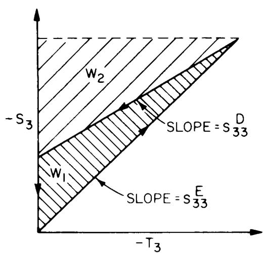
text_image
W₂ -S₃ SLOPE = s₃₃ᴰ W₁ SLOPE = s₃₃ᴱ -T₃
(a)
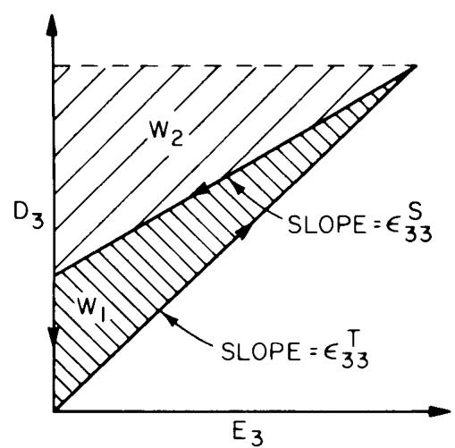
text_image
W₂ D₃ SLOPE = ε₃₃ˢ W₁ SLOPE = ε₃₃ᵀ E₃
(b)
Figure 12—Graphic Illustration of Electromechanical Conversion and Definition of the Piezoelectric Coupling Factor for the Value 0.70 Typical for Piezoelectric Ceramics Used in Transducers (a) Conversion of Energy From a Mechanical Source to Electrical Work (b) Conversion of Energy From an Electrical Source to Mechanical Work
Table 10—Important Static and Quasistatic Coupling Factors
| Material Coupling Factor | Elastic Boundary Condition |
| $k_{31}^{l} = d_{31}/\sqrt{\varepsilon_{33}^{T}s_{11}^{E}}$ | All stress components zero except $T_1$ |
| $k_{33}^{l} = d_{33}/\sqrt{\varepsilon_{33}^{T}s_{33}^{E}}$ | All stress components zero except $T_3$ |
| $k_{36}^{l} = d_{36}/\sqrt{\varepsilon_{33}^{T}s_{36}^{E}}$ | All stress components zero except $T_6$ |
| $k_p = k_{31}/\sqrt{2/(1-\sigma^p)} *$ | All stress components zero except $T_1=T_2$ |
| $k_{31}^{w} = \frac{d_{31}-\frac{s_{12}^{E}}{s_{22}^{E}} d_{32}}{\sqrt{\left(\varepsilon_{33}^{T}-\frac{d_{32}^{2}}{s_{22}^{E}}\right)\left(s_{11}^{E}-\frac{s_{12}^{E^2}}{s_{22}^{E}}\right)}}$ | $T_2, T_1$ only nonzero stress $S_2=0$ |
| $k_{33}^{w} = \frac{d_{33}-d_{31}\frac{s_{13}^{E}}{s_{11}^{E}}}{\sqrt{\left(\varepsilon_{33}^{T}-\frac{d_{31}^{2}}{s_{11}^{E}}\right)\left(s_{33}^{E}-\frac{s_{13}^{E^2}}{s_{11}^{E}}\right)}}$ | $T_3, T_1$ only nonzero stress $S_1=0$ |
| $k_{33}^{t} = e_{33}/\sqrt{c_{33}^{D}\varepsilon_{33}^{S}}$ | $S_3$ only nonzero strain |
| $k_{15}^{t} = e_{15}/\sqrt{c_{55}^{D}\varepsilon_{11}^{S}}$ | $S_5$ only nonzero strain |
NOTE — Only the first four coupling factors exist under static and quasistatic conditions. The others require static constraint that cannot strictly be provided except at resonance and with proper choice of relative dimensions.
in this form holds only for ¥m, 6m, 3m, 3, and 6; .
Domain-wall motion causes energy dissipation, especially at low frequencies, even under low-signal conditions when the motion is reversible. It is therefore found that there is considerable variation in permittivity, compliance, and piezoelectric response with frequency. Variations with frequency are most pronounced with ferroelectric materials having relatively lossy permittivity and compliance. Changes may be as high as 5% per decade of frequency above frequencies of about 1 Hz.
6. Determination of Elastic, Piezoelectric, and Dielectric Constants
6.1 General
The elastic, piezoelectric, and dielectric properties of a piezoelectric material are characterized by a knowledge of the fundamental constants referred to a rectangular coordinate system fixed relative to the crystallographic axes. A determination of these fundamental constants requires a series of measurements on samples of various orientations. There are a number of specific sample geometries and experimental techniques that one can use to make the measurements. The choice of which techniques to employ is subject to many considerations such as the size and shape of samples and the instrumentation available. It is therefore not desirable to specify a single technique for measuring piezoelectric materials. The quantities actually measured nevertheless must be related to the fundamental elastic, piezoelectric, and dielectric constants by procedures that are theoretically sound. This section presents some examples of experimental techniques and the related equations used for the determination of the electroelastic constants.
6.2 Dielectric Constants
The dielectric constants can be evaluated from measurements of the capacitance of plates provided with electrodes covering the major surfaces. These measurements are best made at a frequency substantially lower (´ 0.01 or less) than the lowest resonance frequency of the crystal plate, in which case the measurements yield the dielectric permittivities as constant stress or “free” dielectric permittivities .
In a crystal of the triclinic system there are six dielectric permittivities. From measurements of three plates cut normal to the X, Y, and Z axes, the three dielectric permittivities , and are obtained directly. The remaining three dielectric permittivities , and are found most directly from measurements on three plates rotated about the and Z axes, respectively. In all other crystal systems, fewer than six orientations are necessary.
At frequencies that are high compared to the principal natural frequencies of the plate but well below any ionic resonances, and sufficiently removed from high overtone resonance frequencies, the dielectric permittivities one measures correspond to the constant strain or “clamped” dielectric permittivities . The relations between the dielectric permittivities at constant strain and constant stress are given by Eqs 43, namely,
In practice it is found that the can be measured with somewhat better accuracy than the , primarily because the are measured at low frequencies. For this reason it is recommended that the measured values of be accepted directly and that the be calculated from Eq 126 once the piezoelectric constants are known. Since it is sometimes necessary to know the value of an to calculate a piezoelectric e constant from measured quantities, Eq 126 may have to be solved for the by iteration, particularly if the material in question has low symmetry. In this case it is convenient to use a measured , if possible, to start the iteration.
Measurements of the low-frequency dielectric permittivities are best made on a good quality capacitance bridge and usually are straightforward (see ASTM D150-87 [3]). Some materials present special problems, for example, a material with finite resistivity or a material that has low-frequency dielectric relaxations so that the dielectric permittivities vary with frequency. Occasionally a crystal may have a very large dielectric anisotropy (such as , in which case extreme care must be taken to minimize fringing fields when measuring the smallest dielectric constants. This can be done by using a guard electrode as described in ASTM D150-87 [3], or by making the minor surfaces of the sample flat and perpendicular to the major surfaces and extending the electrodes beyond the edges of the sample by a distance at least five times the sample thickness.
6.3 Static and Quasistatic Measurements
The earliest experimenters with piezoelectric materials determined elastic and piezoelectric constants by static tests. Since it is difficult to control the electrical boundary conditions, static measurements of elastic constants are no longer used for piezoelectric materials. However, static measurements of piezoelectric constants are still used occasionally, and of course, static tests are necessary for determining the positive sense of coordinate axes as described in 3.5.
There has been some confusion regarding the use of static tests for determining the positive sense of axes, so the technique is discussed in some detail here. Consider the plate-shaped sample shown in Fig 13. The major surfaces, which are perpendicular to the axis and are of area A, have electrodes that are shunted by a capacitor with capacitance C. When a uniaxial stress is applied to the sample, the equations governing the resulting charges and fields generated by the stress are as follows:
where t is the sample thickness, q is the charge on the upper plate of the capacitor, V is the potential difference between the upper and lower plates of the capacitor, and it has been assumed that due to the electrodes on the major surfaces. When these equations are solved for V, which is the quantity one usually measures, one obtains
Thus V is positive if and . If C » , Eq 128 reduces to
where is the force applied to the crystal. The signs of the charges and fields shown in Fig 13 are correct for the case and , and are of course reversed i is reversed in sign.
Static measurements [B16] of the magnitudes of piezoelectric constants can be made utilizing either the direct piezoelectric effect or the converse effect. For the direct effect, application of a constant stress under conditions of zero electric fields yields
Eq 130 provides the basis for many techniques for measuring the magnitudes and signs of the constants. The electric field is approximately zero inside a plate-shaped sample with electrodes on the major surfaces that are shunted by a large capacitor. However, if the stress is to be applied to the major surfaces, it is then difficult, due to friction, to ensure that the stress is uniaxial. Thus, as a compromise, the lateral dimensions should be about twice the thickness. additional problem with the use of the direct effect is that some of the charge generated by the application (or removal) of the stress can leak off before it is measured. Drift due to pyroelectric effects causes further confusion with crystals in polar classes.
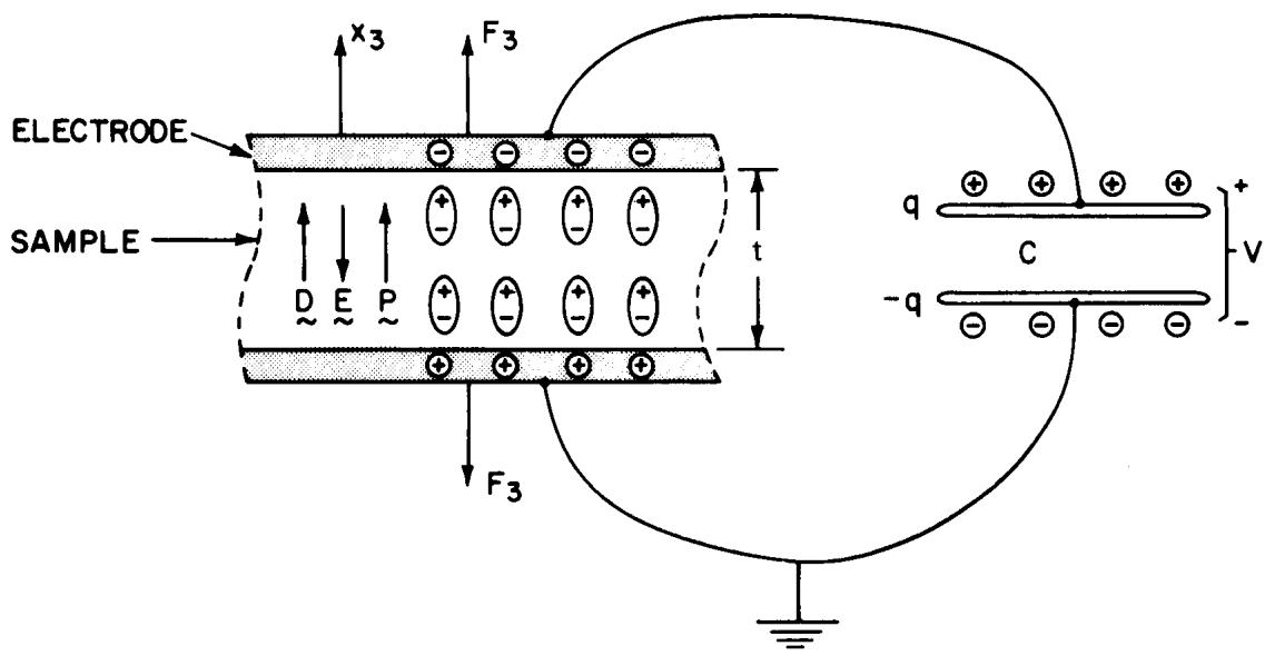
text_image
ELECTRODE SAMPLE x₃ F₃ D E P t F₃ q + + + +
C
q
Figure 13—Signs of Charges and Fields for Static Test of Sample With Under Tension
For the converse effect, application of a constant electric field under conditions of zero stress inside the sample yields
Use of the converse effect is generally more accurate for measuring piezoelectric constants than use of the direct effect, although the small strains produced by an electric field of reasonable size can lead to experimental difficulties. A condition of zero stress within a sample can be assured regardless of its shape, and it is relatively easy to apply a uniform electric field. The strain can be measured with reasonable accuracy, approximately 1%, by means of strain gauges or with interferometric techniques.
Since alternating electric signals eliminate the influence of pyroelectric effects and are more convenient to measure than dc signals, a useful extension of static techniques is made by the application of an alternating stress or electric field to the sample [B16]. As long as the frequency of the applied signal is much less than the fundamental resonance frequency of the sample with its mounting in the test instrument, Eqs 130 and 131 still apply, and improved accuracy can be obtained in this way.
In general, static and quasistatic techniques for measuring piezoelectric constants are capable of reasonable accuracy, a few percent or less under optimum conditions, and have proven useful in certain special cases. One example is routine testing of poled ferroelectric ceramics. These techniques are not recommended in this standard, however, for investigations of new crystals, particularly crystals with low symmetry, because dynamic methods are capable of greater accuracy and can be applied easily to a much wider range of crystal orientations and sample geometries.
6.4 Resonator Measurements
The electrical properties of a piezoelectric vibrator are dependent on the elastic, piezoelectric, and dielectric constants of the vibrator materials. Thus, values for these constants can be obtained from resonator measurements on a suitably shaped and oriented specimen, provided the theory for the mode of motion of that specimen is known. The measurements basically consist of determining the electrical impedance of the resonator as a function of frequency. In principle it is necessary to measure the resonance and antiresonance frequencies, the capacitance, and the dissipation factor well removed from the resonance range to obtain the information required for finding the material constants. In some instances an accurate measurement of the antiresonance frequency cannot be made, and it is then convenient to characterize the resonator by a lumped-parameter equivalent circuit and to calculate the material constants from the measured parameters of this circuit.
6.4.1 The Equivalent Circuit
The impedance properties of a piezoelectrically excited vibrator can be represented near an isolated resonance by a lumped-parameter equivalent circuit, the simplest form of which is shown in Fig 14.
NOTE — The impedance and admittance functions for a piezoelectrically excited vibrator derived in Section 4. often can be represented more exactly by a transmission line equivalent circuit [B17], [B18].
The representation of a piezoelectric vibrator by this circuit is useful only if the circuit parameters are constant and independent of frequency. In general the parameters are approximately independent of frequency only for a narrow range of frequencies near the resonance frequency and only if the mode in question is sufficiently isolated from other modes.
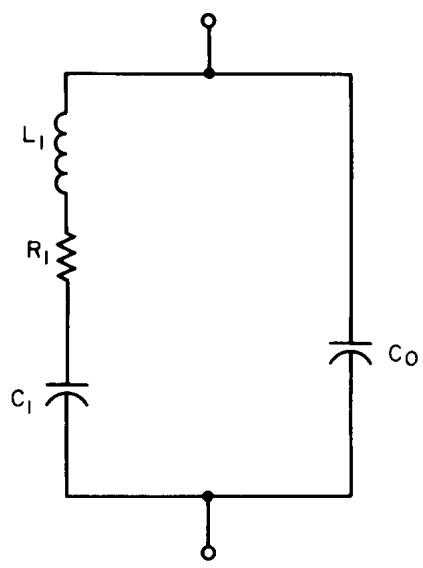
chemical
Simple electrical circuit diagram with inductor, resistor, and capacitor components labeled L1, R1, C1, and C0
Figure 14—Equivalent Electrical Circuit of a Piezoelectric Vibrator
NOTE — The close proximity in frequency of several modes of vibration may be represented by adding additional R-L-C branches in parallel to the branch shown. If the admittance of more than one of these branches is appreciable at a given frequency, difficulties are encountered.
Within this frequency range, the parameters generally approach constant values as the amplitude of vibration approaches zero. The amplitude that can be tolerated before the parameters are appreciably affected varies widely among vibrators of various types and can only be determined by experiment.
The motional resistance in the equivalent circuit represents the mechanical dissipation of the piezoelectric resonator, which is not considered in Sections 2. and 4.. A dimensionless measure of the dissipation is the quality factor Q,
A detailed analysis of the piezoelectric vibrator for which the equivalent circuit of Fig 14 applies is contained in IEEE Std 177-1977 [5].
NOTE — The case of higher mechanical losses where the equivalent circuit is assumed to hold exactly is described in [B19]. An analysis accounting for dielectric, piezoelectric, and elastic losses is described in [B20].
A more complex equivalent circuit which accounts for parasitic elements due to the resonator mounting is treated in [B21]. Every effort should be made to minimize the effects of these parasitic elements in resonators that are constructed for the purpose of measuring material constants.
6.4.2 Effect of Dissipation on the Definition and Measurement of Frequencies Near Resonance and Antiresonance
The resonator theory presented in Section 4. applies to ideal lossless materials, in which case the resonator impedance is purely reactive and the characteristic frequencies and are well defined. The dissipation present in real materials obscures the definition of these frequencies.
Whereas in the lossless resonator there are single frequencies and which coincide with the admittance and impedance maxima, respectively, there are, in a lossy resonator, three frequencies of interest near the admittance maximum and, similarly, three frequencies near the impedance maximum. Accordingly, the critical frequencies and each have three associated frequencies, and corresponding to maximum absolute admittance (impedance), maximum conductance (resistance), and zero susceptance (reactance), respectively. In this standard is defined as the frequency of maximum conductance and is defined as the frequency of maximum resistance. These definitions are independent of the lumped-parameter equivalent circuit.
The relative difference in the frequencies and depends on both the material coupling factor and the resonator geometry. For this reason a quantity called the effective coupling factor has been used, particularly in filter design literature, as a convenient measure of this difference:
Also the resonator figure of merit M is defined here in terms of and as follows:
When is small, this reduces to the definition given M in IEEE Std 177-1978 [5].
The definition given here is equivalent to the definition given as the series resonance frequency of the equivalent circuit in IEEE Std 177-1978 [5]. However, the definition given here is equivalent to the definition given as the parallel resonance frequency in IEEE Std 177-1978 [5] only for resonators with small and high The relations given in IEEE Std 177-1978 [5] among the frequencies , and are accurate only for resonators with small keff.
The critical frequencies of the lossy resonator must correspond to the critical frequencies of an ideal resonator made from a lossless material having the same electroelastic constants as the actual resonator material. That is, if terms accounting for dissipation were introduced into the basic equations of Section 2., and the electrical impedance of the lossy resonator were calculated, the frequencies and would equal the characteristic frequencies obtained in the limit as the dissipative terms approach zero.
For the evaluation of material constants it is always sufficient to substitute an experimental value of for in the equations of Section . For resonators with , an experimental value of is equal within the experimental error in determining the resistance maximum. In general, differs from by about .
For resonators having it is sufficient to use a measured value of or fr directly for , and a measured value of directly for Techniques for measuring and are described in IEEE Std 177-1978 [5], the techniques for measuring and are described in IEC 444 (1973) [4]. When it may be necessary to make corrections to the quantities measured, or to make more detailed measurements on an admittance or impedance bridge to determine and directly as described in [B21]. When the frequency cannot be measured accurately, although can still be measured with reasonable accuracy as long as .
For all equations in the remainder of this section it is assumed that the correspondence and has been made.
6.4.3 The Motional Capacitance Constant and Measurement of the Motional Capacitance
In addition to the frequencies and the motional capacitance of the equivalent circuit is a convenient parameter for relating the resonator response to the elastic, piezoelectric, and dielectric material constants. In this connection it is useful to define the motional capacitance constant , where is the motional capacitance of the vibrator, t is the linear dimension parallel to the direction of the electric field, and A is the electrode area. The quantity G has the same physical dimensions as a permittivity.
Three methods are described here for measuring The first method, which is preferred, is to measure the frequency dependence of the resonator reactance near resonance with an impedance bridge. The points will lie approximately on a straight line and the slope at is related to by
The error in is less than 1% for the resonators with .
A second method is to measure the motional resonance frequency for the combination of a resonator in series with a capacitor plot of versus then yields a straight line with a slope of as shown by the following approximate relation:
Either side of 136 should be greater than 10 for the approximation to be valid. This method is most suitable for resonators with a high figure of merit, , and does not necessarily require the use of a bridge.
The third method, which is suitable for resonators with low figures of merit, is to make separate determinations of the quality factor and the motional resistance . Then is given by the expression
Values for and can be obtained from measurements of the resonator conductance versus frequency on an admittance bridge.
6.4.4 Relations Between Vibrator Response and Material Constants
For each of the modes of vibration analyzed in Section 4. there is a transcendental expression for the electrical impedance that, in the absence of losses, is exact except for the approximations made in obtaining the equation of motion and boundary conditions. Expressions relating the frequencies and to the material constants are obtained from the equations and , respectively.
The proper procedure for obtaining an expression that relates the motional capacitance constant to the material constants is to match the equivalent circuit impedance. (letting for this calculation) and its first derivative to those of the exact impedance at the frequency . Thus, from
one obtains
and from
one obtains
The parallel capacitance in the equivalent circuit is not easily related to the material constants. However, it is never necessary to measure for determining material constants. If one really wants a representative value for of a resonator, for example, for a filter application, one procedure is to find the value that gives the best fit to the correct impedance over the frequency range of interest [B22]. Of course, if the coupling factor is small, 0.1 or less, then can be calculated accurately from the dielectric constant and dimensions of the resonator.
6.4.5 Length-Extensional Modes of Bars
The length-extensional modes of bars [B23] have particular significance for the determination of material constants because these are the only simple modes of vibration for which the material can be an arbitrarily oriented crystal in class 1. Measurements of the length-extensional modes of a sufficient number of independently oriented bars cut from an asymmetric material will result in the determination of the nine elastic compliances:
and six combinations of the remaining twelve compliances:
Here the compliances are or , depending on whether the electric field is applied perpendicular to or parallel to the length of the bar.
For the other crystal systems the number of elastic compliances determinable from measurements on bars decreases with increasing symmetry. Measurements limited to the extensional modes of bars are in no case sufficient to determine all the elastic compliances.
For measurements with the electric field perpendicular to the length of the bar, there are two distinct cases as discussed in 4.5. Referring to Fig 9, only the case with the field applied along the smallest dimension t is recommended for use in determining material constants. In this case the electrical impedance of the resonator is given by
where the quantities appearing in Eq 142 are as defined in 4.5. A measurement of the frequencyE determines the elastic compliance 11 from
The electromechanical coupling factor can be determined from the frequencies and
where or from the motional capacitance constant
where Eq 145 is obtained by substituting Eq 142 into Eq 141. The piezoelectric constant can then be calculated from , and , with its sign found by a static test. Measurements of this type on a sufficient number of independently oriented bars will result in the determination of the nine piezoelectric strain constants:
and six combinations of the other nine constants:
Here, of course, the constants are referred to the crystal axes, and some of them may be zero due to symmetry.
When the electric field is applied parallel to the length of the bar resonator, the electric impedance is given by
where the quantities appearing in Eq 146 are as defined in 4.5. The elastic compliance is determined from the antiresonance frequency by
The electromechanical coupling factor can be obtained from the frequencies and by
or from the motional capacitance constant by
where , and Eq 149 is found by substituting Eq 146 into Eq 141. The expression for G is considerably more complicated here than in the previous case with the field applied perpendicular to the length of the bar. When is less than 0.1, then
is an adequate approximation to Eq 149. Values of the quantity for larger values of are given in Table 11.
Table 11—Motional Capacitance Constants for the Length-Extensional Mode of a Rod and the Thickness Mode of a Plate as a Function of Electromechanical Coupling Factor
| k | $\hat{\beta}_{33}^{T} \Gamma$ | $\Gamma/\in^s$ |
| 0.15 | 0.0183 | 0.0187 |
| 0.20 | 0.0327 | 0.0341 |
| 0.25 | 0.0513 | 0.0548 |
| 0.30 | 0.0744 | 0.0817 |
| 0.35 | 0.1020 | 0.1162 |
| 0.40 | 0.1342 | 0.1598 |
| 0.45 | 0.1715 | 0.2150 |
| 0.50 | 0.2138 | 0.2851 |
| 0.55 | 0.2617 | 0.3752 |
| 0.60 | 0.3153 | 0.4926 |
| 0.65 | 0.3749 | 0.6492 |
| 0.70 | 0.4411 | 0.8649 |
| 0.75 | 0.5141 | 1.1752 |
| 0.80 | 0.5946 | 1.6515 |
| 0.85 | 0.6828 | 2.4606 |
| 0.90 | 0.7794 | 4.1022 |
| 0.95 | 0.8850 | 9.0765 |
The piezoelectric constant can be calculated from , and . Measurements of this type on a sufficient number of independently oriented bars will determine the three piezoelectric constants:
and seven combinations of the remaining fifteen constants:
Before carrying out measurements on bars, it is best to measure first all of the dielectric constants , as outlined in The frequency is always measured for each specimen. However, one has a choice of measuring either the motional capacitance or One important consideration used to make this choice is the sample capacitance. If it is small, then the parasitic capacitance shunting the specimen can be comparable to the sample capacitance. This will cause a measurement of to be erroneous. However, a parasitic shunt capacitance has no effect on measurements of or the motional capacitance. When the sample capacitance is large enough, a measurement o is simpler and is to be preferred.
The bar specimens should be narrow enough to render unimportant any errors due to the influence of the width-length ratio. For measurements of the frequency constants the width-length ratio should be less than 0.1 to approximate the assumed infinitely narrow bar. However, for measurements made to obtain the coupling factor, the width-length ratio can be increased to 0.3 for convenience, since in practice not as much accuracy is required for piezoelectric constants as for elastic constants. The width-thickness ratio should be greater than 2 for measurements with the field perpendicular to the length.
6.4.6 Radial Modes of Disks
A radial mode [B12], [B13], [B24]–[B26] can be excited in disks cut normal to the axis for materials in classes 3m, 6, and 6mm. Due to the difficulty of preparing disks from crystalline specimens, this mode has been used almost exclusively for measurements on poled ferroelectric ceramics. Nevertheless, its importance in this connection warrants coverage in this standard.
From the basic theory of the disk resonator presented in 4.6 one finds that the electrical impedance is given by
where t is the disk thickness, a the radius, and is defined by Eq 112. If is defined as , then is the lowest root of
Table 12 gives the variations of with Thus, from a measurement of the fundamental resonance frequency of a disk resonator, one obtains
Eq 153 is clearly not sufficient to determine either or . One convenient method [B12] to obtain is to measure also the resonance frequency of the first overtone radial mode, given by the second lowest root of 152. The ratio then depends only on and is given as a function of in Table 12. Once is found in this way, may be calculated from Eq 153. Another method for measuring is described in IEC 444 (1973) [4].
is defined as , that ,
then the planar coupling factor can be calculated as follows from measurements of the resonance and antiresonance frequencies:
Table 12—Frequency Constant of Disk Resonator and Ratio of First Overtone to Fundamental Resonance Frequencies as a Function of the Planar Poisson’s Ratio
| $\sigma^p$ | $η_1$ | $f_s^{(2)}/f_s$ |
| 0 | 1.84118 | 2.89566 |
| 0.05 | 1.87898 | 2.84258 |
| 0.10 | 1.91539 | 2.79360 |
| 0.15 | 1.95051 | 2.74826 |
| 0.20 | 1.98441 | 2.70617 |
| 0.25 | 2.01717 | 2.66699 |
| 0.30 | 2.04885 | 2.63043 |
| 0.35 | 2.07951 | 2.59625 |
| 0.40 | 2.10920 | 2.56423 |
| 0.45 | 2.13797 | 2.53416 |
| 0.50 | 2.16587 | 2.50589 |
| 0.55 | 2.19294 | 2.47926 |
| 0.60 | 2.21922 | 2.45414 |
| 0.65 | 2.24434 | 2.43040 |
Figure 15 shows a plot of versus for , and 0.6 as calculated from 155. The coupling factor can be calculated also from a measurement of the motional capacitance constant,
but a measurement of usually is preferable in this case.
The dielectric constant introduced in 4.5 is related to the dielectric constants and by the following expressions:
Thus, for materials in classes 3,3m, 6, and 6mm, the dielectric constants and are related by the simple expression
Also, the planar coupling factor and the extensional mode coupling factor are related by Eq 117, namely,
This last relation provides another technique for measuring
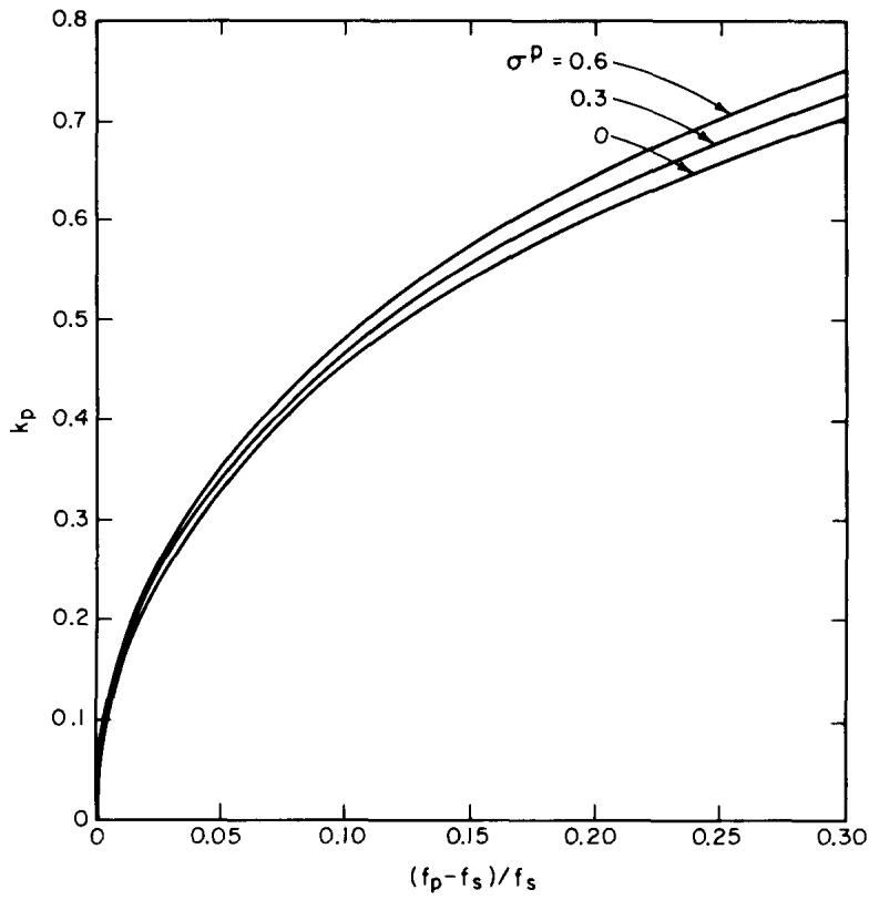
line chart
| (fp-fs)/fs | kp (σ^p = 0.6) | kp (σ^p = 0.3) | kp (σ^p = 0) |
|---|---|---|---|
| 0.0 | 0.1 | 0.1 | 0.1 |
| 0.05 | 0.3 | 0.28 | 0.27 |
| 0.10 | 0.45 | 0.43 | 0.41 |
| 0.15 | 0.55 | 0.53 | 0.51 |
| 0.20 | 0.62 | 0.60 | 0.58 |
| 0.25 | 0.68 | 0.66 | 0.64 |
| 0.30 | 0.72 | 0.70 | 0.68 |
Figure 15—Planar Coupling Factor of Thin Disk Versus for 0.3, and 0.6
In measuring radial-mode resonators one should normally have t < 20a to approximate the assumed infinitely thin disk. However, when one is measuring the first overtone radial mode to determine this condition is not adequate, and one should have to ensure reliable results. The use of Rayleigh-type corrections as discussed in IEEE Std 178-1958 (R1972) [6], is not recommended when the primary intent of the measurement is the determination of material constants.
6.4.7 Thickness Modes of Plates
In general, the thickness modes of plates are quite complex, as discussed in 4.3. For certain crystal symmetries and orientations, however, only a single thickness mode is excited by an electric field in the thickness direction, and measurements on resonators vibrating in these modes are useful for determining certain piezoelectric constants. In particular, a plate whose normal is along a two-, three-, four-, or sixfold axis, and whose plane is not a mirror plane and contains no twofold axis, will vibrate in a pure thickness extensional mode. A plate whose plane contains exactly one twofold axis (this includes , four-, and sixfold axes) will vibrate in a pure thickness shear mode, polarized along the twofold axis.
For both thickness extensional and thickness shear modes, there are three relevant material constants, an elastic constant , a piezoelectric constant and a dielectric constant . The electromechanical coupling factor k is given in terms of these constants by
The elastic constant is related to the frequency
where t is the plate thickness, and the electrical impedance is of the form
where A is the electrode area. From Eq 162 one finds that the coupling factor can be determined from the frequencies and
or from the motional capacitance constant:
When is an adequate approximation to Eq 164, and for values of versus k are given in Table 11.
For some specific examples, a Y-cut quartz plate (class 32) vibrates in a pure thickness shear mode and the relevant constants are , and . A Z-cut cadmium sulfide plate (class 6mm) vibrates in a pure thickness extensional mode and the relevant constants are , and .
In measuring thickness mode resonances, the plate thickness should be 0.1 or less times the smallest transverse dimension. Even if this is the case, coupling to high overtone contour modes is frequently a serious problem. Often the plate dimensions must be changed slightly to get a clear resonance for measuring
Due to the many spurious resonances from high overtone contour modes, it is not desirable to attempt a direct measurement of . It is preferable to determine from high overtone resonances as mentioned in 4.3 and discussed further in 6.5. The coupling factor can then be calculated using Eq 163. An alternative procedure [B10] is to measure the frequencies of the fundamental and first or higher overtone resonances and use the ratio to calculate the coupling factor. For materials with small coupling factors, however, is small, and it may be more accurate to measure the motional capacitance.
6.4.8 Other Modes
IEEE Std 178-1958 (R1972) [6] discussed certain other modes, specifically contour modes of square plates. Since the analysis of these modes involves more severe approximations than those used in this standard, and since the range of validity of these approximations cannot readily be determined in all cases, the use of these modes for measuring material constants is not recommended in this standard.
6.5 Measurement of Plane-Wave Velocities
For piezoelectric materials, the plane-wave velocities, as discussed in 4.2, are related to the fundamental material constants by Eqs 49, 50, and 47, which may be written as follows:
with
The determinantal equation 165 yields three positive real eigenvalues to give the velocities of the three plane waves propagating in the direction n. Thus it is possible, in principle, to determine each of the elastic and piezoelectric tensor elements if one measures the propagation velocities of plane waves for a sufficient number of distinct propagation and particle displacement directions in the solid. One must then find values of the constants that yield the measured velocities when substituted into Eqs 165 and 166.
6.5.1 Pulse-Echo Methods
The term “pulse-echo methods” encompasses those techniques in which the plane-wave velocities are determined from pulse transit time measurements. There are a variety of specific techniques for measurements of this type. The choice of which one to use depends upon whether absolute or relative measurements are wanted, the required accuracy of the velocity measurement, and also upon the properties of the material under consideration. For all the common pulse-echo techniques, a piezoelectric transducer, usually a thin quartz plate, is affixed to the sample to act as a generator and receiver for the propagating stress waves. (Sometimes two transducers are employed in a transmission arrangement where the stress wave is generated at one end of the sample and received at the other end.) A short radiofrequency electrical pulse is applied to the transducer, and a series of pulses is then observed (on an oscilloscope, for example) as the acoustic disturbance is reflected back and forth within the sample. The velocity is then computed from the pulse transit time and the sample thickness (Fig 16). Variations of this basic scheme are available to measure more accurately the time delay between the echoes. With these variations one can compensate for various inaccuracies that can occur, for example, the phase shift in the bond between transducer and sample, the effect of distortion of the pulses during reflection, and so forth. The predominant characteristics of some of the more common techniques are summarized in Table 13 together with references to articles in which the details of a particular method may be found. It is evident from the table that the most accurate methods are those which rely on a pulse interference technique. Several general discussions of ultrasonic velocity measurements are also available [B28], [B35]–[B37].
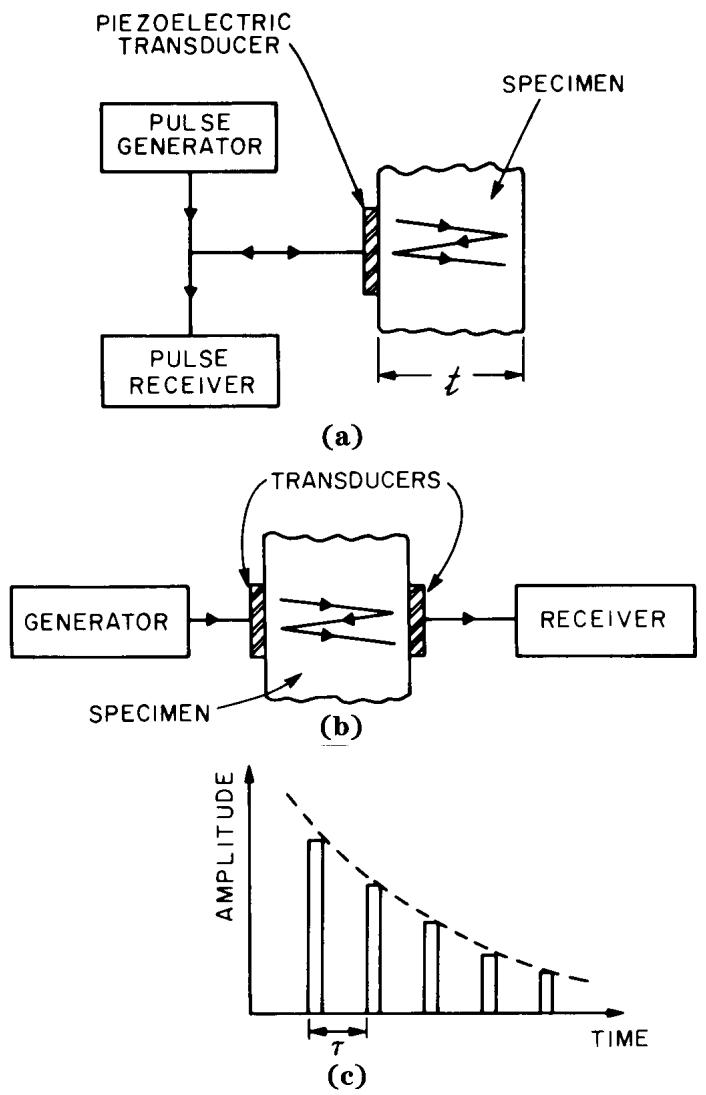
Figure 16—Pulse-Echo Measurement of Velocity (a) Pulse Reflection (b) Pulse Transmission (c) Received Pulse Pattern, Velocity = t/
It should be noted that for plane waves propagating in an arbitrary direction in a crystal, the energy flux vector, defined by Eq 26, generally is not collinear with the propagation direction n. If the deviation is large and the sample dimensions are not much larger than the size of the transducer, some portion or all of the ultrasonic beam may hit the side boundaries before reaching the far end of the sample.
6.5.2 High Overtone Thickness Modes
As indicated in 4.3, the thickness modes of an arbitrarily anisotropic plate are exceedingly complex. While it is possible in principle to extract information about material constants from measurements of the impedance versus frequency near a resonance, it is not practical to do so. Thus, in this case the measurements are restricted to the resonance frequencies of high overtones, in the limits where Eqs 59 and 60 apply. This measurement then yields the plane-wave velocities for waves propagating in the thickness direction of the plate. That is, from Eq 60,
where is the mth overtone resonance frequency of the nth mode, is the plane-wave velocity corresponding to that mode, and t is the plate thickness. The overtone frequencies are high enough when the velocity computed from Eq 167 remains constant to within ±0.1% for three successive values of m.
To measure the high-overtone resonance frequencies, one can use any convenient technique to excite the mode to be measured. Thus, some modes (unstiffened modes) cannot be excited by an electric field in the thickness direction of the plate. One can sometimes excite these modes by an electric field in the plane of the plate (see 4.4), and hence both electrode configurations shown in Fig 17 are useful for these measurements.
Table 13—Common Pulse Measurement Techniques for Ultrasonic Velocity Determinations
| Method | Features | Accuracy | Sensitivity | References |
| Detected pulses | Time delay between successive leading edges of the detected echoes is measured. The required apparatus is relatively simple. | $10^{-2}$ | $10^{-3}$ | Lazarus [B27]McSkimin [B28] |
| Pulses with carrier display | Same as the preceding, except that the delay is found by observing the flat half-cycle of the RF carrier in each echo.Most useful for low-megahertz frequencies in low-loss materials. | $10^{-3}$ | $10^{-5}$ | Forgacs [B29] |
| Pulse superposition or phase cancellation | Either the pulse repetition rate or the carrier frequency is adjusted so as to cause constructive or destructive interference of successive echoes. The accuracy and sensitivity depend upon the apparatus and assume that suitable corrections for transducer and bond have been added. | $10^{-4}$ | $10^{-5}$ | McSkimin [B30]Williams and Lamb [B31]McSkimin and Andreatch [B32], [B33] |
| Sing-around | A detected transmitted pulse is used to trigger the pulse generator for the next pulse. The velocity is then measured by observing the pulse repetition rate. This technique is most useful for measuring small changes in velocity. | $10^{-3}$ | $2 \cdot 10^{-5}$ to $10^{-7}$ | Forgacs [B34] |
The effect of mass loading by the electrodes, discussed in 4.3, is more important for the measurement of high overtone resonances than for any of the other resonator measurements, but this is not found to be a serious problem in practice. If the plate is made with a reasonable thickness (1 mm has been found to be a good choice for many materials), and if a low-density electrode material such as aluminum is used, the resonance frequency reduction due to electrode inertia is easily held to a few parts in .
Finally, it should be noted that measurements of high overtone thickness mode resonances yield exactly the same information as pulse-echo measurements of plane-wave velocities. The velocities measured in this way are accurate to about 1 part in , primarily due to limitations in making the major surfaces of the plates flat and parallel and determining the plate thickness. The accuracy is almost an order of magnitude worse than that obtainable by pulseecho techniques. Hence the pulse-echo methods are preferred if the instrumentation and samples are available to use them.
6.5.3 An Example
Pulse-echo measurements of ultrasonic velocity can be used in conjunction with other experimental techniques to determine the fundamental material constants. Or in some instances, it may be convenient to determine all the constants from the plane-wave velocities. As an example, a procedure for obtaining the constants for a material of class 23 (bismuth germanium oxide, for example) is outlined here. This high symmetry is chosen for simplicity-, a lower symmetry class would require a more complicated analysis. A crystal of this symmetry has three independent elastic constants, one piezoelectric constant, and one dielectric permittivity constant (see Table 8). These five constants can be found from four ultrasonic velocity measurements and one low-frequency capacitance measurement, which determines the permittivity . For propagation in the (100) direction, the longitudinal-wave velocity is , and there are two shear waves, each having the same velocity , where is the density. For propagation in the (011) direction (rotation of the crystal by 45 degrees about the X axis), one measures the velocities of the two shear waves for which (displacement along (100)) and determine all the constants: and are determined directly, is then computed from and the piezoelectric constant is computed from the equations
or
The sign of is positive according to the convention on the choice of axes in Section 3.
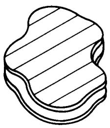
natural_image
Isometric view of a 3D block structure with horizontal stripes, no text or symbols present
(a) Thickness Excitation
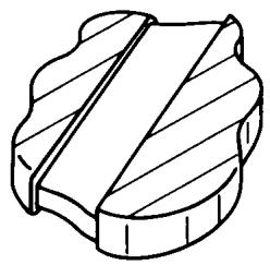
natural_image
Technical drawing of a mechanical part with hatched sections (no text or symbols)
(b) Lateral Excitation
Figure 17—Electrode Configurations for Thickness Vibrations
Notice from Eq 169 that is given in terms of the difference between a stiffened and an unstiffened velocity. If is very small, it cannot be determined accurately in this way. Thus the use of velocity measurements to obtain piezoelectric constants is best suited to cases where the piezoelectric stiffening is large. However, the elastic stiffness constants can be found more accurately from pulse-echo measurements than by any other method.
6.6 Temperature Coefficients of Material Constants
Temperature coefficients of the elastic, piezoelectric, and dielectric constants are important for predicting the variation with temperature of the frequency response of practical resonators and filters. For materials with small electromechanical coupling, such as quartz [B38]–[B40], the piezoelectric and dielectric constants usually have a negligible effect on the temperature response of devices using the material; only the temperature coefficients of the elastic constants and the thermal expansion coefficients are significant. When the electromechanical coupling is large, for example, as in [B41], the temperature coefficients of all constants may be significant.
The nth-order temperature coefficient of the quantity q at the reference temperature is defined by
where so that
Measurements of the type described previously in this section made as a function of temperature are used to obtain the temperature coefficients of material constants. Two methods are available for computing the coefficients from the measurements.
- The equations for ultrasonic velocity or frequency may be differentiated with respect to temperature and the coefficients of the constants explicitly computed from the coefficients of velocities or frequencies.
- The constants may be calculated at each of several temperatures and their coefficients found by curve fitting.
The first method is particularly appropriate either when the material is of high symmetry so that the equations are simple, or when satisfactory results are obtained by neglecting the piezoelectric and dielectric constants. The second method is mathematically simpler but less direct. Ordinarily not more than the lowest two coefficients can be extracted reliably by these methods. An exception occurs when the lowest coefficients become very small for certain specific orientations.
Certain precautions must be observed in the measurement of temperature coefficients. The validity of the power series approximation to the temperature behavior should be tested. If more than two coefficients are needed to fit the data, the possible presence of a phase transition or anomaly due to an impurity should be investigated. The effects of mechanical supports, electrode size, plate geometry, and drive level for resonator measurements should be minimized as far as possible. Anomalous pulse patterns due to irregularities in the sample, transducer, or bond must be avoided in the case of ultrasonic pulse-echo measurements. Such effects may often be detected by comparison of measurements at slightly different frequencies.
Finally, a good test of the derived temperature coefficients is the prediction and confirmation of the temperature behavior of resonators of simple geometry from the fundamental constants.
7. Bibliography
[B1] JEFFREYS, H. Cartesian Tensors. New York: Cambridge University Press, 1931.
[B2] TIERSTEN, H. F. Linear Piezoelectric Plate Vibrations. New York: Plenum Press, 1969.
[B3] MASON, W. P. Piezoelectric Crystals and Their Application to Ultrasonics. New York. Van Nostrand, 1950, p 34.
[B4] KENNARD, O. Primary Crystallographic Data. Acta Crystallographica, vol 22, 1967, p 445.
[B5] International Union of Crystallography. International Tables for X-Ray Crystallography. Birmingham, England: Kynoch Press, 1965.
[B6] BECHMANN, R. Elastic and Piezoelectric Constants of Alpha-Quartz. Physical Review, vol 110, 1958, pp 1060–1061.
[B7] BIRSS, R. R. Symmetry and Magnetism. Amsterdam: North Holland, 1964.
[B8] MASON, W. P. Crystal Physics of Interaction Processes. New York: Academic Press, 1966, p 309.
[B9] MINDLIN, R. D. Thickness-Shear and Flexural Vibrations of Crystal Plates. Journal of Applied Physics, vol 22, 1951, p 316. MINDLIN, R. D. Waves and Vibrations in Isotropic Elastic Plates, in Structural Mechanics. London: Pergamon, 1960, pp 199–232. MINDLIN, R. D., and GAZIS, D. C. Strong Resonances of Rectangular AT-Cut Quartz Plates. Proceedings of the 4th US National Congress of Applied Mechanics, 1962, pp 305–310.
[B10] ONOE, M., TIERSTEN, H.F., and MEITZLER, A. H. Shift in the Location of Resonant Frequencies Caused by Large Electromechanical Coupling in Thickness-Mode Resonators. Journal of the Acoustical Society of America, vol 35, 1963, pp 36–42.
[B11] WARNER, A., ONOE, M., and COQUIN, G.A. Determination of Elastic and Piezoelectric Constants for Crystals in Class 3m. Journal of the Acoustical Society of America, vol 42, 1967, p 1223.
[B12] MEITZLER, A. H., O’BRYAN, H. M., Jr, and TIERSTEN, H. F. Definition and Measurement of Radial Mode Coupling Factors in Piezoelectric Ceramic Materials With Large Variations in Poisson’s Ratio. IEEE Transactions on Sonics and Ultrasonics, vol SU-20, July 1973, pp 233–239.
[B13] MASON, W. P. Electrostrictive Effect in Barium Titanate Ceramics. Physical Review, vol 74, 1948, p 1134.
[B14] ONOE, M. Tables of Modified Quotients of Bessel Functions of the First Kind for Real and Imaginary Arguments. New York. Columbia University Press, 1958.
[B15] TOUPIN, R. A. The Elastic Dielectric. Journal of Rational Mechanical Analysis, vol 5, 1956, p 849. TIERSTEN, H. F. On the Nonlinear Equations of Thermoelectroelasticity. International Journal of Engineering Science, vol 9,197 1, p 587.
[B16] MASON, W. P., and JAFFE, H. Methods for Measuring Piezoelectric, Elastic, and Dielectric Constants of Crystals and Ceramics. Proceedings of the IRE, vol 42, June 1954, pp 921–930.
[B17] MASON, W. P. Electromechanical Transducers and Wave Filters. New York: Van Nostrand, 1948, p 399.
[B18] REDWOOD, M., and LAMB, J. On the Measurement of Attenuation and Ultrasonic Delay Lines. Proceedings of the IEEE, vol 103, pt B, Nov 1956, pp 773–780.
[B19] MARTIN, G. E. Determination of Equivalent Circuit Constants of Piezoelectric Resonators of Moderately Low Q by Absolute-Admittance Measurement. Journal of the Acoustical Society of America, vol 26, May 1954, pp 413– 420.
[B20] MARTIN, G.E. Dielectric, Elastic, and Piezoelectric Losses in Piezoelectric Materials. Proceedings of the 1974 Ultrasonics Symposium, Milwaukee, WI, Nov 11–14, IEEE Catalog No 74CHO 896-1 SU, pp 613–617.
[B21] HAFNER, E. The Piezoelectric Crystal Unit —Definitions and Methods of Measurement. Proceedings of the lEEE, vol 57, Feb 1969, pp 179–201.
[B22] HANNON, J.J., LLOYD, P., and SMITH, R.T. Lithium Tantalate and Lithium Niobate Piezoelectric Resonators in the Medium Frequency Range with Low Ratios of Capacitance and Low Temperature Coefficients of Frequency. IEEE Transactions on Sonics and Ultrasonics, vol SU-17, Oct 1970, pp 239–246.
[B23] BERLINCOURT, D. Piezoelectric Crystals and Ceramics, in Ultrasonic Transducer Materials, O. E. Mattiat, Ed. New York: Plenum Press 1971, pp 63–124.
[B24] BAERWALD, H. G. Electrical Admittance of a Circular Ferroelectric Disk. Office of Naval Research, Contract Nonr 1055(00), Technical Report 3, Jan 1955. US Department of Commerce, Office of Technical Services, PB 119233.
[B25] ONOE, M. Contour Vibrations of Isotropic Circular Plates. Journal of the Acoustical Society of America, vol 28, Nov 1956, pp 1158–1162.
[B26] McMAHON, G.W. Measurement of Poisson’s Ratio in Poled Ferroelectric Ceramic Disks. IEEE Transactions on Ultrasonics Engineering, vol UE-10, Sept 1963, pp 102–103.
[B27] LAZARUS, D. The Variation of the Adiabatic Elastic Constants of KCl, NaCl, CuZn, Cu, and Al with Pressure to 10,000 Bars. Physical Review, vol 76, Aug 1949, pp 545–553.
[B28] McSKIMIN, H. J. Notes and References for the Measurement of Elastic Moduli by Means of Ultrasonic Waves. Journal of the Acoustical Society of America, vol 33, May 1961, pp 606–615.
[B29] FORGACS, R.L.A System for the Accurate Determination of Ultrasonic Velocity in Solids. Proceedings of the National Electronics Conference, vol 14, Oct 1958, pp 528–543.
[B30] McSKIMIN, H. J. Pulse Superposition Method for Measuring Ultrasonic Wave Velocities in Quartz. Journal of the Acoustical Society of America, vol 33, Jan 1961, pp 12–16.
[B31] WILLIAMS, J., and LAMB, J. On the Measurements of Ultrasonic Velocity in Solids. Journal of the Acoustical Society of America, vol 30, Apr 1958, pp 308–313.
[B32] McSKIMIN, H. J., and ANDREATCH, P. Analysis of the Pulse Superposition Method for Measuring Ultrasonic Wave Velocities as a Function of Pressure and Temperature. Journal of the Acoustical Society of America, vol 34, May 1962, pp 609–615.
[B33] McSKIMIN, H. J., and ANDREATCH, P. Measurements of Very Small Changes in the Velocity of Ultrasonic Waves in Solids. Journal of the Acoustical Society of America, vol 41, Apr 1967, pp 1052–1057.
[B34] FORGACS, R. L. Improvements in the Sing-Around Technique for Ultrasonic Velocity Measurements. Journal of the Acoustical Society of America, vol 32, Dec 1960, pp 1697–1695.
[B35] KYAME, J. J. Wave Propagation in Piezoelectric Crystals. Journal of the Acoustical Society of America, vol 21, May 1949, pp 159–167.
[B36] McSKIMIN, H. J. Ultrasonic Methods for Measuring the Mechanical Properties of Liquids and Solids, in Physical Acoustics, vol 1, pt A, W. P. Mason, Ed. New York: Academic Press, 1969, pp 271–334.
[B37] TRUELL, R., ELBAUM, C, and CHICK, B. B. Ultrasonic Methods in Solid State Physics. New York: Academic Press, 1969, ch 2.
[B38] BECHMANN, R. The Temperature Coefficients of the Natural Frequencies of Piezoelectric Quartz Plates and Bars. Hochfrequenz und Electroakustik, vol 44, 1934, pp 145–160.
[B39] KOGA, I. Thermal Characteristics of Piezoelectric Oscillating Quartz Plates. R. R. R. W. Japan, vol 4,1934, pp 61–76.
[B40] MASON, W.P. Quartz Crystal Applications. Bell System Technical Journal, vol 22, July 1943, pp 178–223.
[B41] SMITH, R. T., and WELSH, F. S. Temperature Dependence of the Elastic, Piezoelectric, and Dielectric Constants of Lithium Tantalate and Lithium Niobate. Journal of Applied Physics, vol 42, May 1971, pp 2219–2230.